Implicit Collaborative Filtering with PySpark
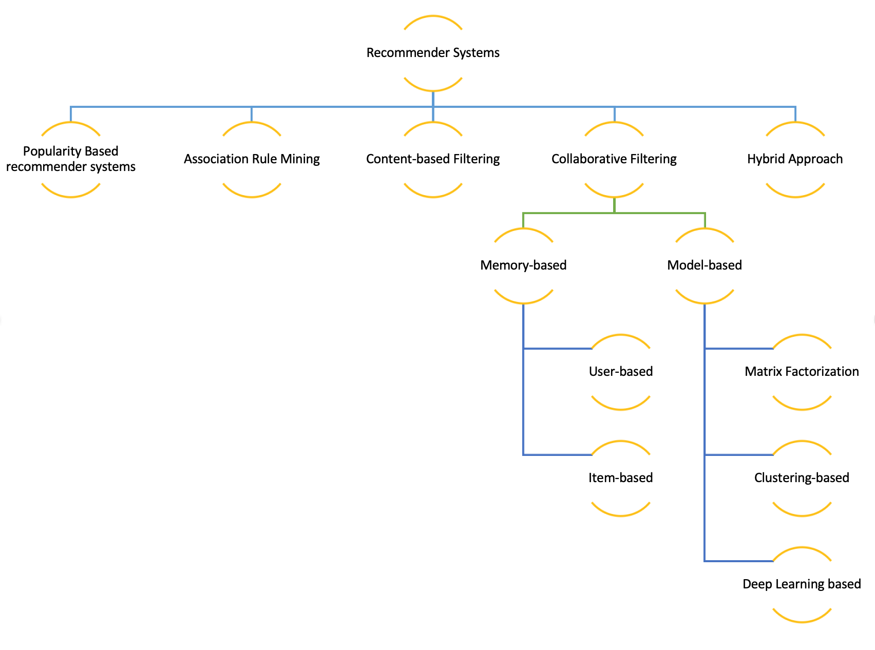
 A recommender system analyzes data, on both products and users, to make item suggestions to a given user, indexed by u, or predict how that user would rate an item, indexed by i. They can be classified based on the approach used for recommendation. Most popular ones include popularity based recommendation systems, association rule mining, content-based filtering, collaborative filtering and hybrid methods. The method one chooses to recommend, relies heavily on the kind of input (implicit vs explicit feedback), data sparsity, scalability and efficiency. Every method has its own advantages and drawbacks.
Before proceeding any further with the methods used to build recommender systems, lets pitch in to discuss the topics like implicit and explicit feedback systems, data sparsity and cold-start problem. Explicit feedback systems refers to the systems where we can use ratings provided by users directly. This is preferred when available, because its more reliable due to absence of any sort of inference. Its not always available, as users are not always prepared to provide it. In contrast, implicit feedback systems interprets rating from user purchase history, navigation history, session duration, content of e-mail and button clicks, among others. This is easily available, because it needs no effort from user.
Furthermore, issues of data sparsity and cold-start problem are quite important to address when building a recommender system. Cold-start problem refers to the issue of recommending an item when you have never seen how that item interacts with other users. This can occur when new users or items are added to the system with little or no ratings. Then, there is the problem of data sparsity. Data sparsity refers to the number of cells in a table that are empty(sparsity) and that contain information(density). It is quite important to note that, the accuracy of the recommender system is affected by the data sparsity and the cold-start problem by a considerable amount.
Popularity based recommendation systems
The popularity-based recommendation system utilizes the data available on top movie review websites to recommend the most popular movies to users based on their star ratings, thus increasing content consumption. Although this kind of recommendation system is simple to implement and scalable, it does not provide personalization to the user. Additionally, since the data that this kind of system relies upon is purely based on the ratings provided on the rating websites, it might not reflect user preferences or account regional dialect of every user.
Association Rule Mining
Association rule mining (also called as Market Basket Analysis), at a basic level, is a rule-based method that analyzes for patterns of co-occurrences, in a database(also called Basket Data). It identifies frequent if-then associations called association rules which consists of an antecedent (if) and a consequent (then). An example of an association rule based on basket data is that 90% of people who watch Star Wars and The Empire Strikes Back! in a given week , also watch A New Hope later that week. This method is greatly useful when user choices are not easily accessible. For example, companies that do not have an online presence uses association rule mining to study purchase patterns and placing the frequently bought items in the same aisle. Although the analysis is easy to understand and interpret, the method can get computationally expensive for large datasets.

As user preferences became easily accessible, recommender systems have been developed to embed user choice and behavior patterns into the algorithms. The other two approaches, content-based filtering and collaborative filtering employs the usage of customer preferences in their algorithms.
Content-based filtering
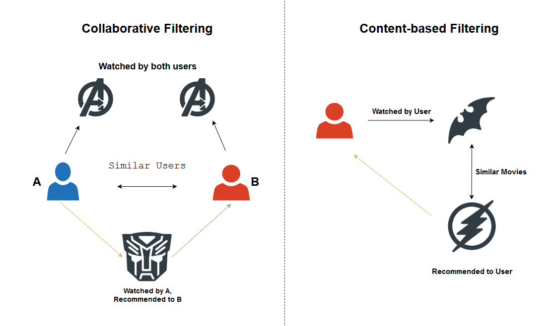
A content-based filtering technique analyzes the past choices of a user and constructs profiles based on the user actions alone to build a preference profile, instead of pairing users with the products that similar users liked. The main advantages of this method is that, it is unaffected by the cold-start problem or user preference changes, and is more explainable since it doesn’t try to infer hidden user preferences. However, they do overspecialize recommendations and users may begin to only receive recommendations similar to the items that they have already encountered.
Collaborative filtering
Collaborative filtering is one of the most popular algorithms for recommender systems. It analyzes interactions or similarity between users and items and is distinct because it looks at the behavior of multiple customers cross-referencing their purchase histories with each other. Good personalized recommendations enhances the user experience, thereby improving customer satisfaction and loyalty. This technique is generally more accurate than content-based filtering. This is because this technique analyzes user preferences and uses these for providing personalized recommendations to other similar users.
Hybrid approach
The hybrid approach of recomender systems use a combination of any of the above-mentioned techniques and other machine learning techniques much like the Graph Recommender and Regression approach.
Implementation of Collaborative filtering
Collaborative filtering can be further divided into memory-based and model-based collaborative filtering. The memory-based approach uses user rating data to compute similarity between users or items. Memory-based systems are not always as fast and scalable as we would like them to be, especially in the context of actual systems that make real-time recommendations on the basis of large datasets.
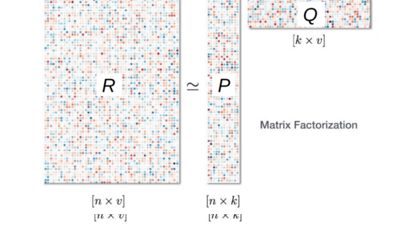
Although there are a number of algorithms that can be used to build the model in model-based approach, one of the most popular ones is the Matrix Factorization technique. Matrix factorization achieves collaborative filtering by approximating an incomplete rating matrix using the product of two matrices in a joint latent factor space of dimensionality f. Before we can get into further details of matrix factorization we will describe some key elements of this technique: The rating matrix, latent factors and the latent vectors. A rating matrix is a matrix of u(users) by i(items) of explicit user ratings over items. This is generally sparse because, not all users could have watched all movies. An entry in this sparse matrix corresponds to the rating, given by user u, of an item i. The latent vector of factors are inferred features from movie rating patterns of users, and are estimated by minimizing the loss function. Examples for latent factors in the context of movies, can be genre, depth of a character, amount of action, age group of the target audience or can even be completely uninterpretable. These inferred features are often called latent vectors and the k attributes are often called the latent factors. Furthermore, the expressive power of the model can be tuned by modifying the number of latent factors.
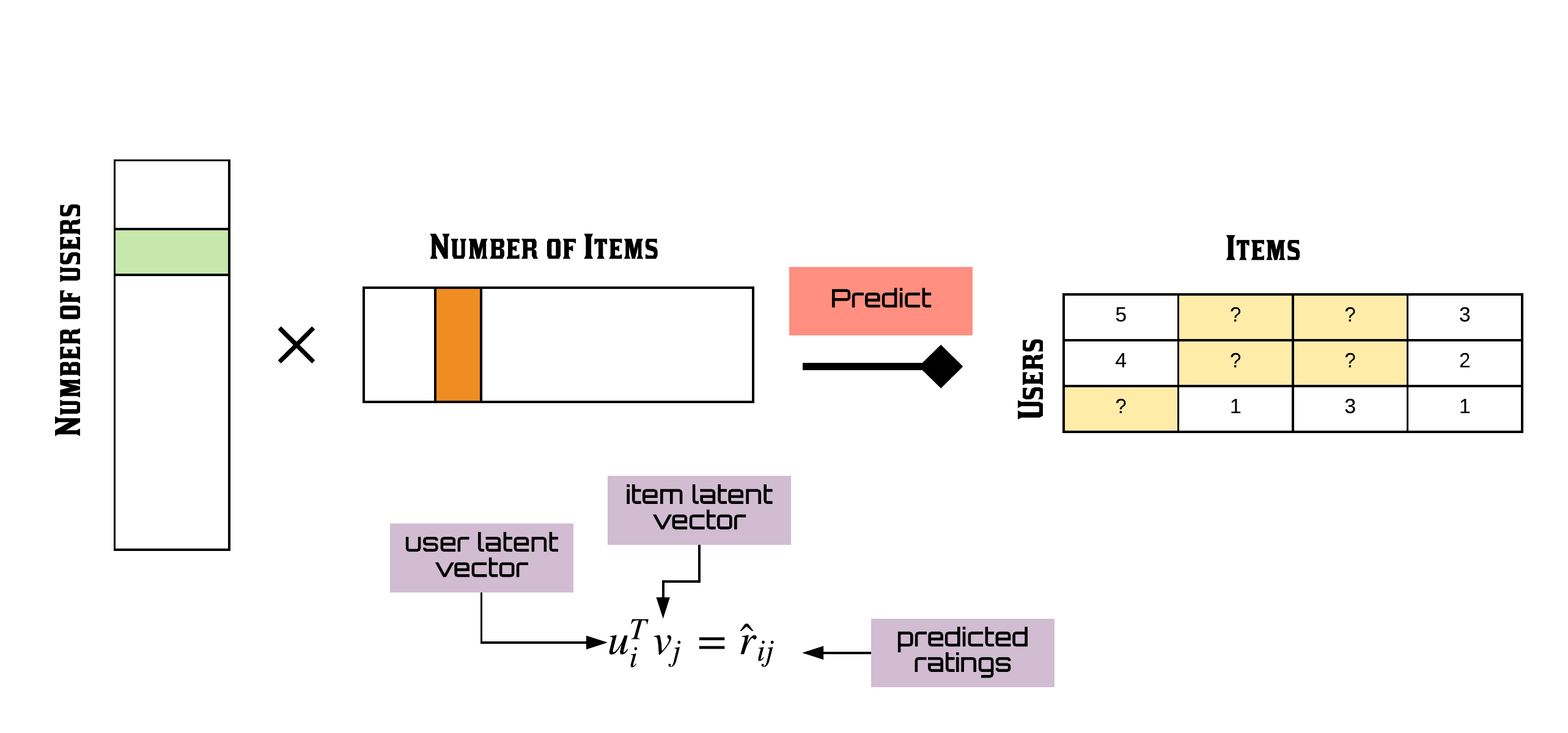
In this article, we will build our movie recommender system with one of the sophisticated algorithms which is more efficient and appropriate for recommender systems : Matrix Factorization. Matrix factorization achieves collaborative filtering by approximating an incomplete rating matrix using the product of two low-rank matrices.
We have used Apache Spark in our recommendation system since it overcomes the hurdle of scalability by implementing Alternating Least Squares to achieve collaborative filtering by matrix factorization technique. Let’s begin with data ingestion and exploration. To load the data as a spark dataframe, import pyspark and instantiate a spark session.
# Creating spark session
from pyspark.sql import SparkSession
from pyspark.conf import SparkConf
from pyspark.sql import functions as f
from pyspark.sql.types import *

spark = SparkSession.builder.appName("movierecommender") \
.config(conf=SparkConf([('spark.executor.memory', '16g'),
                        ('spark.app.name', 'Spark Updated Conf'),
                        ('spark.executor.cores', '6'),
                        ('spark.cores.max', '6'),
                        ('spark.driver.memory','16g')])) \
.getOrCreate()
Data Source:
The data used in this analysis is from the MovieLens 10M set, containing 10000054 ratings and 95580 tags applied to 10681 movies by 71567 users of the online movie recommender service MovieLens. The data is made available by GroupLens, a research group in the Department of Computer Science and Engineering at the University of Minnesota.
# Loading data
movies = spark.read.format("csv").option("header", "false").load("../Data/movierecommender/movies.dat",inferSchema="true")
ratings = spark.read.format("csv").option("header", "false").load("../Data/movierecommender/ratings.dat",inferSchema="true")

movies =(movies
 .withColumn("movieId",f.split("_c0","::").getItem(0).cast("double"))
 .withColumn("title",f.split("_c0","::").getItem(1))
 .withColumn("genres",f.split("_c0","::").getItem(2))
 .select("movieId","title","genres")
)#.show(truncate=False)

ratings = (ratings
.withColumn("userId",f.split("_c0","::").getItem(0).cast("double"))
.withColumn("movieId",f.split("_c0","::").getItem(1).cast("double"))
.withColumn("rating",f.split("_c0","::").getItem(2).cast("double"))
.withColumn("timestamp",f.to_timestamp(f.from_unixtime(f.split("_c0","::").getItem(3))))
.select("userId","movieId","rating","timestamp")
 )#.show(truncate=False)
# Preprocessing data for exploratory data analysis
movielens = ratings.join(movies,["movieId"],"left")
movielens.summary().show()
+-------+-----------------+------------------+------------------+--------------------+------------------+
|summary|          movieId|            userId|            rating|               title|            genres|
+-------+-----------------+------------------+------------------+--------------------+------------------+
|  count|         10000054|          10000054|          10000054|            10000054|           7650044|
|   mean|4120.291476526027| 35869.85940925919| 3.512421932921562|  22.166750376695127|              null|
| stddev|8938.402117920627|20585.337354677813|1.0604184716263587|   32.00949399851806|              null|
|    min|              1.0|               1.0|               0.5|"Great Performanc...|(no genres listed)|
|    25%|            648.0|           18115.0|               3.0|                20.0|              null|
|    50%|           1834.0|           35728.0|               4.0|                20.0|              null|
|    75%|           3627.0|           53598.0|               4.0|                20.0|              null|
|    max|          65133.0|           71567.0|               5.0|            Âge d'or|           Western|
+-------+-----------------+------------------+------------------+--------------------+------------------+
# Final Schema for dataset
movielens.printSchema()
root
 |-- movieId: double (nullable = true)
 |-- userId: double (nullable = true)
 |-- rating: double (nullable = true)
 |-- timestamp: timestamp (nullable = true)
 |-- title: string (nullable = true)
 |-- genres: string (nullable = true)
Train-Validation Split
We then create a 80/20 train-validation split of the movielens dataset for model evaluation purposes. The model is created and trained on the train set and tested on the validation set.
# Train set test set split
(train_set,temp) = movielens.randomSplit([8.0,1.0],seed=1)
# Make sure userId and movieId in validation set are also in train set (to avoid Cold Start Problem)
validation_set = (temp
    .join(train_set,["userId"],"left_semi")
    .join(train_set,["movieId"],"left_semi"))

removed = (temp
 .join(validation_set,["movieId","userId"],"left_anti")
)

train_set = train_set.union(removed)
Exploratory Data Analysis
Data ingestion is followed by data exploration where we intend to gain some insights about the dataset we just loaded. We study each attribute and its characteristics like name, type, percentage of missing values, outliers, type of distribution and many others. The subsequent tasks include studying correlations between the attributes and identifying the promising transformations if needed. Data visualization is quite an important tool for accomplishing these tasks. We document all these intuitions thus obtained by summarizing and visualizing the dataset, aiding the understanding of the project.
With an initial glance of the movielens dataset, we observe that movie information is available in movieId and title columns; user information is available in userId column, timestamp is measured in seconds with “1970-01-01 UTC” as origin; rating column is our target variable; Each movie rating has been categorized into one or more genres which is available in genres column.
# Visualization Libraries
import seaborn as sns
import matplotlib.pyplot as plt
from statsmodels.distributions.empirical_distribution import ECDF
%matplotlib inline
plt.rcParams["figure.figsize"] = (10,8)
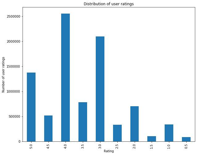
Rating
# Distribution of user ratings
ratings_hist=(train_set
 .groupBy(f.col("rating")).count()
 .sort(f.col("rating").desc())
).toPandas()

ratings_hist.plot.bar("rating","count")
plt.title("Distribution of user ratings")
plt.xlabel("Rating")
plt.ylabel("Number of user ratings")
plt.legend().remove()
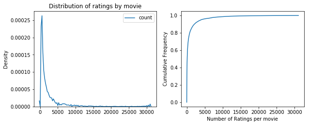
MovieId & Title
# Density Distribution and normalized ECDF of ratings grouped by movie
movies_ratings =(train_set
 .groupBy(f.col("movieId")).count()
).toPandas()

plt.subplot(2, 2, 1)
sns.kdeplot(movies_ratings["count"])
plt.xlabel("")
plt.ylabel("Density")
plt.title("Distribution of ratings by movie")

plt.subplot(2,2,2)
plt.plot(ECDF(movies_ratings["count"]).x,ECDF(movies_ratings["count"]).y)
plt.xlabel("Number of Ratings per movie")
plt.ylabel("Cumulative Frequency")
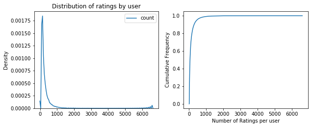
UserId
# Density Distribution and normalized ECDF of ratings grouped by user
user_ratings =(train_set
 .groupBy(f.col("userId")).count()
).toPandas()

plt.subplot(2, 2, 1)
sns.kdeplot(user_ratings["count"])
plt.xlabel("")
plt.ylabel("Density")
plt.title("Distribution of ratings by user")

plt.subplot(2,2,2)
plt.plot(ECDF(user_ratings["count"]).x,ECDF(user_ratings["count"]).y)
plt.xlabel("Number of Ratings per user")
plt.ylabel("Cumulative Frequency")
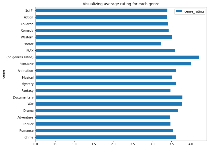
Genres
# Average rating of movies based on genre
avg_genre_rating = (train_set
.select("movieId","userId","genres","rating")
.withColumn("genres_array", f.split("genres", "\|"))
.withColumn("genre", f.explode("genres_array"))
.groupBy("genre").agg(f.mean(f.col("rating")).alias("genre_rating"),
f.countDistinct("movieId").alias("num_movies"),
f.countDistinct("movieId","userId").alias("num_ratings"))
).toPandas()
avg_genre_rating.plot.barh("genre","genre_rating")
plt.title("Visualizing average rating for each genre")
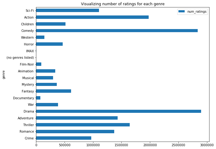
avg_genre_rating.plot.barh("genre","num_ratings")
plt.title("Visualizing number of ratings for each genre")
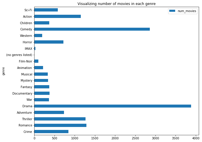
avg_genre_rating.plot.barh("genre","num_movies")
plt.title("Visualizing number of movies in each genre")
Timestamp
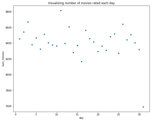
# Analyzing day of the month - Timestamp of rating
day_month_rating = (train_set
.withColumnRenamed("timestamp","date")
.withColumn("day",f.dayofmonth(f.col("date")))
.groupBy("day").agg(f.mean(f.col("rating")).alias("avg_rating"),
f.countDistinct("movieId").alias("num_movies"),
f.countDistinct("movieId","userId").alias("num_ratings"))
).toPandas()
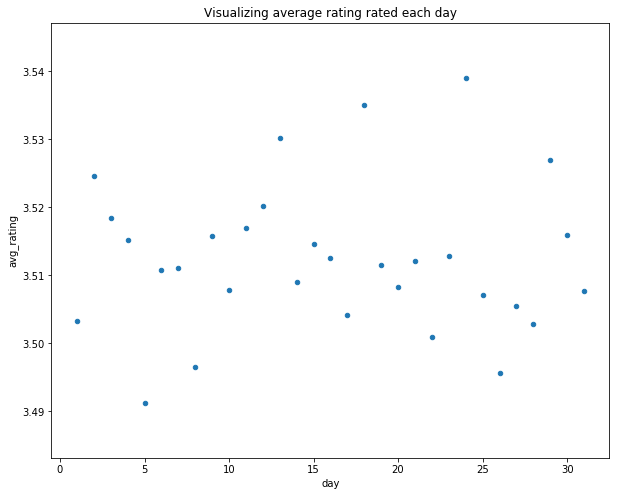
day_month_rating.plot.scatter("day","avg_rating")
plt.title("Visualizing average rating rated each day")
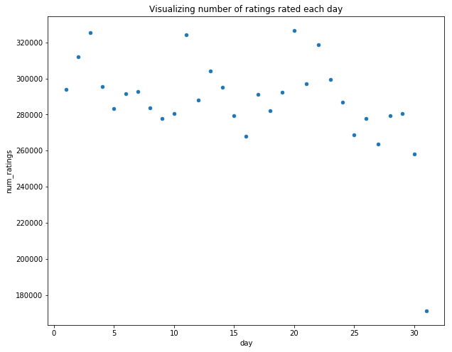
day_month_rating.plot.scatter("day","num_ratings")
plt.title("Visualizing number of ratings rated each day")
day_month_rating.plot.scatter("day","num_movies")
plt.title("Visualizing number of movies rated each day")
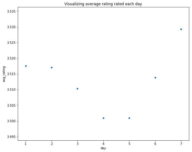
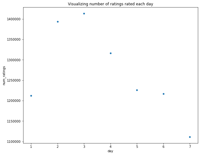
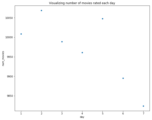
# Analyzing day of the week - Timestamp of rating
day_week_rating = (train_set
 .withColumnRenamed("timestamp","date")
 .withColumn("day",f.dayofweek(f.col("date")))
 .groupBy("day").agg(f.mean(f.col("rating")).alias("avg_rating"),
                     f.countDistinct("movieId").alias("num_movies"),
                     f.countDistinct("movieId","userId").alias("num_ratings"))
).toPandas()

day_week_rating.plot.scatter("day","avg_rating")
plt.title("Visualizing average rating rated each day")
day_week_rating.plot.scatter("day","num_ratings")
plt.title("Visualizing number of ratings rated each day")
day_week_rating.plot.scatter("day","num_movies")
plt.title("Visualizing number of movies rated each day")
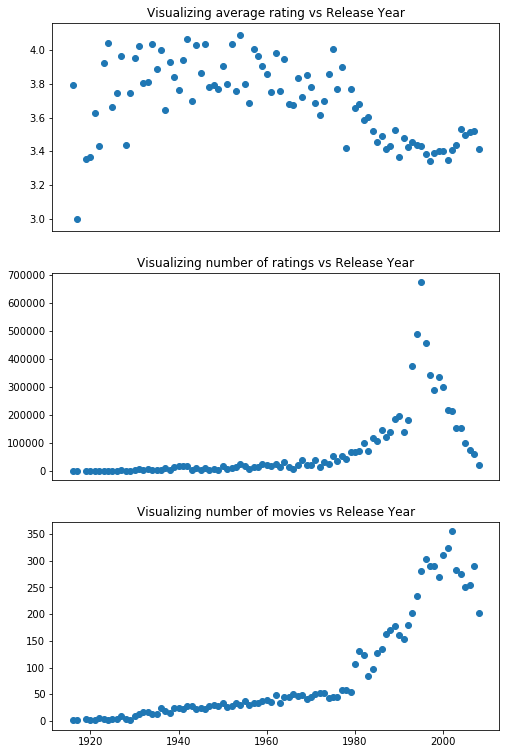
Release Year
release_year_rating = (train_set
 .select("title","movieId","userId","rating")
 .withColumn("releaseyear",f.substring('title',-5,4))
 .filter(f.col("releaseyear")>1900)
 .groupBy("releaseyear").agg(f.mean(f.col("rating")).alias("avg_rating"),
                             f.countDistinct("movieId").alias("num_movies"),
                             f.countDistinct("movieId","userId").alias("num_ratings"))
).toPandas()

plt.figure(figsize=(8,13))
plt.subplot(3, 1, 1)
plt.scatter(release_year_rating.releaseyear.astype('int64'),release_year_rating.avg_rating)
plt.title("Visualizing average rating vs Release Year")
plt.xticks([])
plt.subplot(3, 1, 2)
plt.scatter(release_year_rating.releaseyear.astype('int64'),release_year_rating.num_ratings)
plt.title("Visualizing number of ratings vs Release Year")
plt.xticks([])
plt.subplot(3, 1, 3)
plt.scatter(release_year_rating.releaseyear.astype('int64'),release_year_rating.num_movies)
plt.title("Visualizing number of movies vs Release Year")
Building a recommender system using ALS
from pyspark.ml.recommendation import ALS
from pyspark.ml.evaluation import RegressionEvaluator
# Basic Model parameters
als = ALS(
        userCol = "userId",
        itemCol = "movieId",
        ratingCol = "rating",
)
# Evaluator
evaluator = RegressionEvaluator(
    metricName = "rmse",
    labelCol = "rating",
    predictionCol = "prediction"
)
# Fit and Transform
model = als.fit(train_set)
predictions = model.transform(validation_set)
rmse = evaluator.evaluate(predictions.na.drop())
print(rmse)
0.8145315605180299
from pyspark.ml.tuning import CrossValidator, ParamGridBuilder

# Creating Hyperparameter grid for tuning the model
parameter_grid = (
    ParamGridBuilder()
    .addGrid(als.rank ,[1,5,10])
    .addGrid(als.maxIter,[20])
    .addGrid(als.regParam,[0.05,0.1])
    .build()
)

# Cross validation on the hyperparameter grid
crossvalidator = CrossValidator(
    estimator=als,
    estimatorParamMaps=parameter_grid,
    evaluator=evaluator,
    numFolds=2,
)
# Model fitting and predictions
crossval_model = crossvalidator.fit(train_set)
predictions = crossval_model.transform(validation_set)
rmse = evaluator.evaluate(predictions)
print(rmse)
0.8704685337508209
opt_model = crossval_model.bestModel
opt_model
ALS_486e13132101
Recommendations for All users
In this section, we generate recommendations based on the requirements.
Recommendations can be generated for all users, a list of users, or a single user.
# Recommending top 10 movies for all users
recommend_all_users = model.recommendForAllUsers(10).cache()
recommend_all_users.show(20,False)
+------+-----------------------------------------------------------------------------------------------------------------------------------------------------------------------------------------------------+
|userId|recommendations                                                                                                                                                                                      |
+------+-----------------------------------------------------------------------------------------------------------------------------------------------------------------------------------------------------+
|148   |[[25975, 5.4700174], [32657, 5.346849], [65001, 5.2740993], [33264, 5.2295647], [64275, 5.110407], [42783, 5.102586], [53883, 5.102167], [4454, 5.0949736], [26048, 5.0001564], [58898, 4.9635277]]  |
|463   |[[32657, 4.847002], [65001, 4.7771854], [25975, 4.4827065], [1198, 4.405077], [318, 4.396311], [260, 4.368013], [858, 4.3357124], [1196, 4.307836], [527, 4.2753315], [33264, 4.2257524]]            |
|471   |[[61037, 5.360802], [6691, 5.2161136], [7113, 5.199141], [5910, 5.0650325], [65133, 5.0478106], [31692, 4.9775057], [61253, 4.962686], [63772, 4.9039984], [31053, 4.885498], [5280, 4.8721533]]     |
|496   |[[6256, 5.5736775], [32444, 5.3224363], [3233, 4.932787], [58898, 4.8912807], [6026, 4.873434], [8794, 4.8674264], [65001, 4.8434134], [53883, 4.817717], [61037, 4.8133693], [25975, 4.7717247]]    |
|833   |[[32657, 5.202602], [65001, 5.166078], [25975, 4.893692], [33264, 4.7185593], [42783, 4.7057843], [858, 4.680309], [318, 4.6259556], [64275, 4.593347], [53883, 4.585396], [4454, 4.5681868]]        |
|1088  |[[32657, 4.3691797], [65001, 4.305023], [42783, 4.289133], [25975, 4.268764], [33264, 4.265427], [64275, 4.225163], [26048, 4.099648], [53883, 4.0805454], [4454, 4.0606704], [63310, 4.0098634]]    |
|1238  |[[65001, 5.064704], [32657, 4.921974], [6691, 4.790737], [33264, 4.5722423], [25975, 4.5702443], [4454, 4.544714], [63310, 4.5401587], [318, 4.530655], [527, 4.5174904], [42783, 4.472168]]         |
|1342  |[[32657, 4.9682355], [65001, 4.9285536], [25975, 4.9068804], [53883, 4.8117256], [42783, 4.786216], [33264, 4.5924845], [53355, 4.589077], [858, 4.5875235], [64275, 4.583851], [4454, 4.542359]]    |
|1580  |[[42783, 4.8741136], [32657, 4.7512918], [65001, 4.530798], [64280, 4.507534], [60983, 4.4713836], [53883, 4.4679813], [4171, 4.459224], [61742, 4.446425], [64275, 4.4205337], [33264, 4.4109383]]  |
|1591  |[[31692, 6.0121784], [61037, 5.9581733], [65133, 5.8372254], [6511, 5.820645], [32444, 5.7605586], [65001, 5.5315375], [7113, 5.492081], [31053, 5.424225], [6691, 5.3908563], [64990, 5.3305492]]   |
|1645  |[[65001, 5.2055397], [32657, 4.87617], [63310, 4.833739], [6691, 4.7939863], [4454, 4.742594], [25975, 4.647519], [63772, 4.635081], [42783, 4.6163015], [7144, 4.611266], [33264, 4.5727134]]       |
|1829  |[[8519, 5.554109], [6511, 5.51192], [31692, 5.260827], [61037, 5.166402], [61253, 5.0205665], [6256, 4.998061], [65133, 4.9973607], [7113, 4.9345074], [1852, 4.9337997], [6914, 4.8441997]]         |
|1959  |[[65001, 4.5332794], [61037, 4.3907313], [63310, 4.244684], [7144, 4.218011], [32657, 4.165986], [65133, 4.104204], [63772, 4.099427], [27841, 4.0865903], [8794, 4.066941], [25975, 4.006586]]      |
|2122  |[[42783, 4.0203156], [53883, 3.8283653], [65001, 3.8283324], [25975, 3.8157954], [4454, 3.8106773], [32657, 3.805549], [64275, 3.722776], [33264, 3.7216868], [61742, 3.7030056], [53355, 3.6560252]]|
|2142  |[[58898, 4.3103175], [25975, 4.248044], [53883, 4.1045313], [5194, 4.0838985], [61037, 4.010985], [65001, 4.0035443], [7113, 3.9833894], [33451, 3.9700255], [6098, 3.9644954], [51209, 3.9581857]]  |
|2366  |[[65001, 5.6398244], [61037, 5.5232506], [8659, 5.323239], [63310, 5.320412], [7113, 5.3039894], [7144, 5.2929325], [65133, 5.26829], [27841, 5.2605104], [63772, 5.2384663], [4454, 5.235513]]      |
|2659  |[[2319, 5.230588], [6691, 5.179285], [61037, 5.174231], [61253, 5.0963936], [7113, 4.9791565], [620, 4.958443], [65133, 4.9479938], [7144, 4.9030876], [25975, 4.901422], [8037, 4.8883734]]         |
|2866  |[[60983, 5.1214347], [53883, 4.9311247], [58898, 4.8760796], [4454, 4.6970935], [25975, 4.6436796], [42783, 4.6420755], [6026, 4.541827], [64275, 4.4280224], [62336, 4.400916], [33264, 4.387739]]  |
|3175  |[[6691, 5.454208], [65001, 5.36091], [32657, 5.0101976], [4454, 4.999255], [25975, 4.993573], [63310, 4.9743776], [7113, 4.9255896], [33264, 4.879459], [7140, 4.846695], [32444, 4.8386354]]        |
|3749  |[[32657, 5.083437], [65001, 4.990966], [42783, 4.933362], [32444, 4.8663697], [33264, 4.6988335], [25975, 4.6623864], [64275, 4.6188536], [26048, 4.613469], [858, 4.6009183], [53883, 4.5495605]]   |
+------+-----------------------------------------------------------------------------------------------------------------------------------------------------------------------------------------------------+
only showing top 20 rows
Detailed recommendation for the selected user
# Checking movie title from the previous generated recommendations
USER_ID = 1238
(
    recommend_all_users
    .filter(f"userId == {USER_ID}")
    .withColumn("rec",f.explode("recommendations"))
    .select("userId",
            f.col("rec").movieId.alias("movieId"),
            f.col("rec").rating.alias("rating"),
           )
    .join(movies,"movieId")
    .orderBy("rating",ascending=False)
    .select("movieId","title")
).show(truncate=False)
+-------+-------------------------------------+
|movieId|title                                |
+-------+-------------------------------------+
|65001  |Constantine's Sword (2007)           |
|32657  |Man Who Planted Trees                |
|6691   |Dust (2001)                          |
|33264  |Satan's Tango (Sátántangó) (1994)    |
|25975  |Life of Oharu                        |
|4454   |More (1998)                          |
|63310  |War Lord                             |
|318    |Shawshank Redemption                 |
|527    |Schindler's List (1993)              |
|42783  |Shadows of Forgotten Ancestors (1964)|
+-------+-------------------------------------+
Recommendation for a particular user based on predictions for unwatched movies
# Consider any random user from the userId
USER_ID = 1238

# Movies not rated by the selected user
movies_to_be_rated = (
    ratings
    .filter(f"userId != {USER_ID}")
    .select("movieId").distinct()
    .withColumn("userId",f.lit(USER_ID))
)
# Predictions on unwatched movies only
user_movie_preds = model.transform(movies_to_be_rated)
user_movie_preds.show()

# Movie recommendations for userId - Manually feeding unwatched movies
(user_movie_preds
.dropna()
.orderBy("prediction",ascending = False)
.limit(10)
.join(movies,["movieId"])
.select("userId","movieId","title",f.col("prediction").alias("rating"))
.orderBy("rating",ascending = False)
).show(truncate=False)
+-------+------+----------+
|movieId|userId|prediction|
+-------+------+----------+
|  148.0|  1238| 2.7894876|
|  463.0|  1238| 2.7958498|
|  471.0|  1238| 3.5524511|
|  496.0|  1238| 2.8227122|
|  833.0|  1238|  2.266191|
| 1088.0|  1238| 3.4465244|
| 1238.0|  1238|  3.844698|
| 1342.0|  1238|  2.479726|
| 1580.0|  1238| 3.6329877|
| 1591.0|  1238| 2.2646801|
| 1645.0|  1238| 3.2694008|
| 1829.0|  1238| 2.7408764|
| 1959.0|  1238| 3.7475433|
| 2122.0|  1238| 2.1890275|
| 2142.0|  1238| 3.0301836|
| 2366.0|  1238| 3.4558885|
| 2659.0|  1238| 3.1594718|
| 2866.0|  1238| 3.6068923|
| 3175.0|  1238| 3.6340725|
| 3749.0|  1238| 2.9524477|
+-------+------+----------+
only showing top 20 rows

+------+-------+-------------------------------------+---------+
|userId|movieId|title                                |rating   |
+------+-------+-------------------------------------+---------+
|1238  |65001.0|Constantine's Sword (2007)           |5.064704 |
|1238  |32657.0|Man Who Planted Trees                |4.921974 |
|1238  |6691.0 |Dust (2001)                          |4.790737 |
|1238  |33264.0|Satan's Tango (Sátántangó) (1994)    |4.5722423|
|1238  |25975.0|Life of Oharu                        |4.5702443|
|1238  |4454.0 |More (1998)                          |4.544714 |
|1238  |63310.0|War Lord                             |4.5401587|
|1238  |318.0  |Shawshank Redemption                 |4.530655 |
|1238  |527.0  |Schindler's List (1993)              |4.5174904|
|1238  |42783.0|Shadows of Forgotten Ancestors (1964)|4.472168 |
+------+-------+-------------------------------------+---------+
It is seldom the case that one algorithm is enough to make real world recommendations. Its important to address all the issues we discussed and more. In reality, the algorithms used in real world are mostly hybrid and is tailored to the needs of the recommender system needed.
I hope you enjoyed reading!!