Detecting Fraudulent Transactions in Credit Cards

Introduction
Nowadays, artificial intelligence(AI) is being used in all realms of business. One such interesting application of machine learning is online fraud detection. With increased sophistication and scale of fraudulent transactions, fraud detection has become one of the indispensable tool for every organization. The conventional approaches to fighting online fraud include predictive models and are rule based. These are no longer effective at tackling advanced levels of current fraud attempts. Online fraud detection needs AI to stay well ahead of the current sophistication of fraudsters. This motivates the need to build a fraud detection system.
IEEE-CIS Fraud Detection Dataset
The dataset used in this analysis comes from Kaggle competition, IEEE Fraud Detection-CIS 2019 Technical Challenge. The data on kaggle is broken into two files identity and transaction, which are joined by TransactionID. Not all transactions have corresponding identity information. The data is collected by Vesta’s fraud protection system and digital security partners. Vesta Corporation is the forerunner in guaranteed e-commerce payment solutions. Founded in 1995, Vesta pioneered the process of fully guaranteed card-not-present (CNP) payment transactions for the telecommunications industry.
However, the data used in this analysis is the training dataset provided for this competition. The test set was not used in this analysis since we do not have labels for evaluating the performance on the test set. The purpose of this analysis is to predict the probability that an online transaction is fraudulent, as denoted by the binary target isFraud.
The following is a summary of features of the dataset.
Outcome variable :
- isFraud : Binary target variable (0 : Legitimate, 1 : Fraud)
Categorical Features :
- ProductCD: product code, the product for each transaction.
- card1 - card6: payment card information, such as card type, card category, issue bank, country, etc.
- addr1, addr2: address
- P_emaildomain: purchaser email domain
- R_emaildomain: recipient email domain
- M1-M9: match, such as names on card and address, etc.
- DeviceType
- DeviceInfo
- id_12 - id_38 : identity information – network connection information (IP, ISP, Proxy, etc) and digital signature (UA/browser/os/version, etc) associated with transactions.
Numeric Features :
- TransactionDT: timedelta from a given reference datetime (not an actual timestamp).
- TransactionAMT: transaction payment amount in USD.
- dist1, dist2: distance
- C1-C14: counting, such as how many addresses are found to be associated with the payment card,etc. (The actual meaning is masked.)
- D1-D15: timedelta, such as days between previous transaction, etc.
- Vxxx: Vesta engineered rich features, including ranking, counting, and other entity relations.
- id_01 - id_11 : identity information.
Loss Functions
Machine learning models are evaluated by means of a loss function. The loss function evaluates the performance of each model and the metric is chosen depending on the kind of task involved in machine learning. Since the main goal of our project is binary classfication (i.e. two possible classes 0 or 1), we will focus on metrics commonly used for binary classifiers. Accuracy and ROC are the most commonly used evaluation metrics for binary classifiers.
However, when the dataset is imbalanced, it is very easy to achieve high accuracy just by classifying everything to the majority class. For example, in fraud detection datasets, majority of the transactions are legitimate and the models can achieve higher accuracy just by classifying all the transactions as legitimate. Therefore, we choose AUC for calibrating our models.
AUC(Area Under Receiver Operating Characteristic Curve)
One of the most commonly used metric to visualize the performance of a binary classifier, is the Receiver Operating Characteristic Curve(ROC) and Area Under Curve(AUC) is the best way to summarize its performance in a single number. Here, the curve refers to the ROC curve.
Project Checklist
Evidently, the first step in building a machine learning model involves framing the problem and getting the data. Then, we choose an appropriate performance metric to rightly assess our models. These metrics are also called loss functions. This is followed by data exploration and data visualization tasks. We then proceed to data preprocessing. There are various tasks involved in this stage from feature selection to handling missing data, encoding the data and splitting the data appropriately. Once this is completed, the next step is generally termed as the prototyping phase, where we train and test various candidate models and select the best model using model selection. The main task of prototyping phase is to select the model. This is followed by hyperparameter tuning, for optimizing our loss function. Once we are satisfied with our prototype model, the same is deployed in production to put it through further testing on live data.
Methods and Analysis
Data Ingestion
In this stage, we download the data and prepare the dataset to be used in the analysis. The dataset is split into two datasets: df and validation with 90% and 10% of the original dataset respectively. We take the validation set and put it off to the side, pretending that we have never seen it before.
#### Create df set, validation set (final hold-out test set)
# Note: this process could take a couple of minutes
if(!require(plyr)) install.packages("plyr", repos = "http://cran.us.r-project.org")
if(!require(tidyverse)) install.packages("tidyverse", repos = "http://cran.us.r-project.org")
if(!require(caret)) install.packages("caret", repos = "http://cran.us.r-project.org")
if(!require(data.table)) install.packages("data.table", repos = "http://cran.us.r-project.org")
if(!require(lubridate)) install.packages("lubridate", repos = "http://cran.us.r-project.org")
if(!require(utils)) install.packages("utils", repos = "http://cran.us.r-project.org")
if(!require(reshape2)) install.packages("reshape2", repos = "http://cran.us.r-project.org")
if(!require(ipred)) install.packages("ipred", repos = "http://cran.us.r-project.org")
if(!require(e1071)) install.packages("e1071", repos = "http://cran.us.r-project.org")
if(!require(pROC)) install.packages("pROC", repos = "http://cran.us.r-project.org")
if(!require(xgboost)) install.packages("xgboost", repos = "http://cran.us.r-project.org")
if(!require(DMwR)) install.packages("DMwR", repos = "http://cran.us.r-project.org")
if(!require(vip)) install.packages("vip", repos = "http://cran.us.r-project.org")
if(!require(randomForest)) install.packages("randomForest", repos = "http://cran.us.r-project.org")
library(plyr)
library(tidyverse)
library(caret)
library(data.table)
library(utils)
library(lubridate)
library(pROC)
library(ipred)
library(e1071)
library(xgboost)
library(reshape2)
library(xgboost)
library(DMwR)
library(vip)
library(randomForest)
# Download files from dropbox link
dl <- tempfile()
download.file("https://dl.dropboxusercontent.com/s/05kl7ogmpsx044j/ieee_cis_fraud_detection.zip", dl)
identification <- read_csv(unzip(dl, "ieee_cis_fraud_detection/train_identity.csv"))
transactions  <- read_csv(unzip(dl, "ieee_cis_fraud_detection/train_transaction.csv"))
fraud_det_set <- transactions %>%
  left_join(identification,by="TransactionID")
# Validation set will be 10% of fraud_det_set data
set.seed(1, sample.kind="Rounding")
test_index <- createDataPartition(y = fraud_det_set$isFraud, times = 1, p = 0.1, list = FALSE)
df <- fraud_det_set[!row.names(fraud_det_set) %in% test_index,]
validation <- fraud_det_set[row.names(fraud_det_set) %in% test_index,]
validation_y <- select(validation,isFraud)
validation_x <- select(validation,-isFraud)
# Removing unwanted objects
rm(dl,identification, transactions,fraud_det_set,test_index,validation)
Create Helper Functions
In this section, we will create the helper functions needed for this dataset for analysis and performance evaluation of models. The following code creates necessary helper functions for this project.
##### Create Helper Functions
# This function creates one-hot encoded columns of a selected column
one_hot_encoding <- function(df,colname){
  # Get the list of possible values category can have
  possible_val <- unique(df[[colname]])
  temp_df <- cbind(sapply(possible_val, function(g) {
    as.numeric(str_detect(df[[colname]], g))
  })
  )
  return(temp_df)
}
# This function performs label encoding of the column passed
label_encoding <- function(df,colname){
  levels <- sort(unique(df[[colname]]))
  temp_df <- as.integer(factor(df[[colname]], levels = levels))
  return (temp_df)
}
# This function replaces multiple values of a column with a single value
replace_columnval <- function(col,multiple,single){
  temp <- replace(col,str_detect(col,paste(multiple,collapse = "|")),single)
  return (temp)}
Exploratory Data Analysis
Outcome - isFraud
The response variable of this analysis is the isFraud variable. A value of 0 denotes that a transaction is fraud and 1 denotes that the transaction is legitimate.
# Class Distribution of Fraudulent vs Legitimate Transactions
ggplot(data = df, aes(x = factor(isFraud), fill = factor(isFraud))) +
  geom_bar(aes(y = (..count..)/sum(..count..)),position = "dodge",alpha=0.7) +
  geom_text(aes(y = (..count..)/sum(..count..),
                label = paste0(..count..," ","  (",round(prop.table(..count..) * 100,2), '%',")")),
            stat = 'count',
            position = position_dodge(.9),
            size=2.5,vjust = -0.3) +
  scale_fill_manual("",values=c("#66c2a5","#fc8d62"),labels=c("Legitimate","Fraud")) +
  labs(x = "", y = '') +
  scale_y_continuous(labels = scales::percent) +
  theme(legend.position = "bottom",
        axis.text=element_blank(),
        axis.ticks = element_blank())
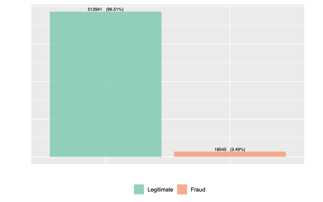
Figure 1 displays the class distribution of the transactions. We observe that, the dataset is not relatively balanced. The fraudulent transactions constitute only a small fraction of the dataset. Using this dataset as the basis for our algorithms, without deploying any techniques for balancing the dataset, can lead to errors due to overfitting. This is because the machine learning models tend to classify all transactions as legitimate to increase the accuracy. Hence, we have to appropriately balance the data before feeding it to the models.
Quantitative Variables
There are 384 quantitative predictor variables in our dataset. The following sections discuss each of the variables in detail.
Transaction ID
The transaction ID is the unique identifier of each observation in our dataset.
Transaction time delta
The TransactionDT variable in our dataset gives the transaction timedelta from a given reference datetime. It does not denote an actual timestamp. The following code visualizes the total transaction amount plotted versus the timedelta for every 24 hour period from the origin.
# TransactionDT : timedelta from a given reference datetime (not an actual timestamp)
# Visualizing days from origin and associated total transaction amount
df %>%
  dplyr::mutate(Day = round(df$TransactionDT/86400)) %>%
  select(isFraud,TransactionAmt,TransactionDT,Day) %>%
  group_by(isFraud,Day) %>%
  dplyr::summarise(txn_amt = sum(TransactionAmt)/1000) %>%
  ggplot(aes(Day,txn_amt,color = factor(isFraud))) +
  geom_point() +
  geom_smooth() +
  scale_color_manual("",values=c("#66c2a5","#fc8d62")) +
  facet_grid(rows = vars(isFraud),
             scales = "free",
             labeller = labeller(isFraud = c("0"= "Legitimate","1" = "Fraud"))) +
  labs(x ="24-hour timedelta Relative from Origin",y="Total Transaction Amount (in Thousands)") +
  theme(legend.position = "none")
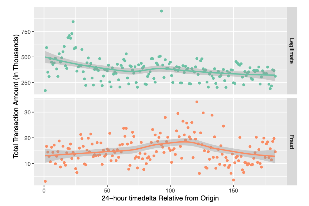
Figure 2 illustrates a subtle variation in total transaction amount in a 24-hour timedelta period. Moreover, the variation is similar for both legitimate and fraudulent transactions.
Transaction amount
One of the most important details about a transaction is the transaction amount. The following code displays the distribution of transaction amount for legitimate and fraud transactions.
### Transaction Amount : transaction payment amount in USD
# Distribution of Transaction amount by fraudulent vs legitimate transactions
df %>%
  ggplot(aes(TransactionAmt,color = factor(isFraud))) +
  geom_density() +
  facet_wrap(vars(isFraud),
             scales = "free",
             labeller = labeller(isFraud = c("0"= "Legitimate","1" = "Fraud"))) +
  scale_color_manual("",
                     values=c("#66c2a5","#fc8d62")) +
  labs(y = "Density",x = "Transaction Amount (in USD)") +
  coord_cartesian(clip = "off") +
  theme(plot.title = element_text(hjust = 0.5,face="italic"),
        legend.position = "none")
# Normalized ecdf of transaction amount of Fraudulent transactions vs Legitimate transactions
df %>%
  ggplot(aes(x = TransactionAmt,
             y =100*..y..,
             color=factor(isFraud))) +
  stat_ecdf(geom = "step",
            size = 0.75,
            pad = FALSE) +
  facet_wrap(vars(isFraud),
             scales = "free",
             labeller = labeller(isFraud = c("0"= "Legitimate","1" = "Fraud"))) +
  scale_x_continuous(breaks = seq(0,30000,5000)) +
  scale_color_manual("",values=c("#66c2a5","#fc8d62")) +
  labs(x = "Transaction Amount (in USD)", y = "Cumulative Frequency") +
  coord_cartesian(clip = "off") +
  theme(legend.position = "none")
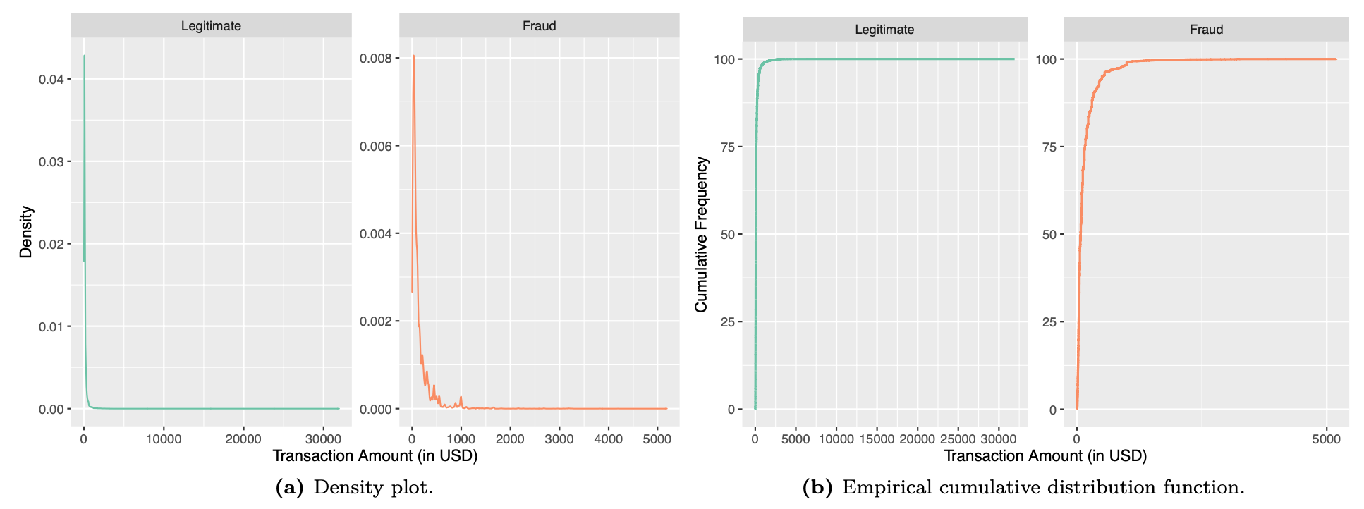
Figure 3 displays the density plot and the ECDF plot for the distribution of the transaction amount. The distribution is a right skewed distribution, with a few transactions with large amount, but the majority of transactions have transaction amount less than 2000 USD for legitimate transactions and 300 USD for fraudulent transactions.
Distance
We proceed to analyze the distance variable. The below code generates a normalized ECDF for the distance values.
### dist1 and dist2 : Distance
# Visualizing dist1 and dist2 values
df %>%
  select(dist1,dist2,isFraud) %>%
  gather("Dist","Values",-isFraud) %>%
  ggplot(aes(Values,color = factor(isFraud))) +
  stat_ecdf(geom = "step",
            size = 0.75,
            pad = FALSE) +
  scale_color_manual("",values=c("#66c2a5","#fc8d62")) +
  facet_grid(isFraud~Dist,
             scales = "free",
             labeller = labeller(isFraud = c("0"= "Legitimate","1" = "Fraud"))) +
  labs(x="Distance",y = "Cumulative Frequency") +
  theme(legend.position = "none")
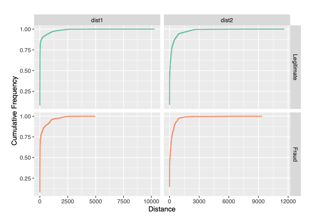
We observe that, a majority of the transactions have missing distance values for dist2. However, the dist1 values are missing for 60% of the transactions. According to figure 4, only a quarter of transactions have distance values for dist1 approximately more than 200 for fraudulent transactions.
C1~C14
The variables C1 to C14 denote counting, such as how many addresses are found to be associated with the payment card,etc. The actual meaning of the variable is masked. To analyze this variable, we can examine the pairwise correlation of the variables C1~C14.
### C1~C14 variables dataframe : counting, such as how many addresses are found to be associated with the payment card,etc.
c_vars_df <-select(df,names(df)[str_detect(names(df),"^C[0-9]+")])
# Pairwise Correlation heatmap of C1~C14
cor(c_vars_df,
     use="pairwise.complete.obs") %>%
  melt() %>%
  dplyr::mutate(Var1=as.numeric(gsub("C([0-9]+)","\\1",Var1)),
         Var2=as.numeric(gsub("C([0-9]+)","\\1",Var2))) %>%
  ggplot(aes(factor(Var1),factor(Var2),fill=value)) +
  geom_tile() +
  scale_fill_gradient2(low = "#d7301f",mid="white", high = "#045a8d") +
  labs(x="",y="") +
  scale_x_discrete(labels =function(x) paste0("C",x)) +
  scale_y_discrete(labels =function(x) paste0("C",x))
# Redundant features among C1~C14
c_vars_drop <- names(c_vars_df)[!str_detect(names(c_vars_df),"C([1,3,5,13]$)")]
# Remove unwanted variables
rm(c_vars_df)
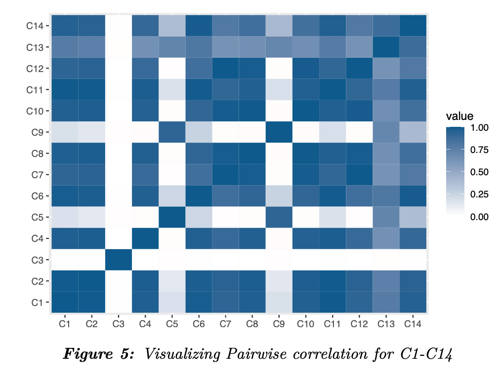
The heatmap in figure 5 illustrates the pairwise correlation between the C1~C14 variables. We see that, there is a strong correlation between many of the variables. Therefore, we consider the variables C1, C3, C5 and C13. We will exclude all other variables from our analysis.
D1~D15
The variables D1 to D15 gives the timedelta, such as days between previous transaction, etc. We perform a similar approach as before and generate a pairwise correlation heatmap for the variables D1~D15. Additionally, we eliminate the columns which have more than 85% missing data.
### D1 ~ D15 : timedelta, such as days between previous transaction, etc.
# D1 ~ D15 variables dataframe
d_vars_df <- select(df,names(df)[str_detect(names(df),"^D[0-9]+")])
# Pairwise Correlation heatmap of D1~D15
cor(d_vars_df,
    use="pairwise.complete.obs") %>%
  melt() %>%
  dplyr::mutate(Var1=as.numeric(gsub("D([0-9]+)","\\1",Var1)),
         Var2=as.numeric(gsub("D([0-9]+)","\\1",Var2))) %>%
  ggplot(aes(factor(Var1),factor(Var2),fill=value)) +
  geom_tile() +
  scale_fill_gradient2(low = "#d7301f",mid="white", high = "#045a8d") +
  labs(x="",y="") +
  scale_x_discrete(labels =function(x) paste0("D",x)) +
  scale_y_discrete(labels =function(x) paste0("D",x))
# Remove variables with more than 85% values missing
d_vars_missingvalues <-
  data.frame(Var = names(colMeans(is.na(df))),
             missingPercent = colMeans(is.na(df))) %>%
  filter(grepl("^D([0-9]+)",Var)) %>%
  filter(!round(missingPercent,2) < 0.85) %>%
  pull(Var)
# Remove unwanted variables
rm(d_vars_df)
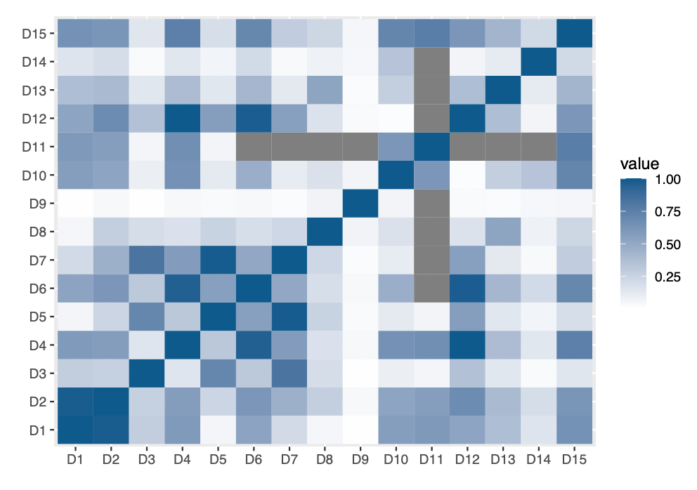
Figure 7: Visualizing pairwise correlation for Vesta engineered rich features
The heatmap in figure 6 does not show a strong correlation between any of the variables. The variables with more than 85% of missing values will be dropped from analysis.
Vxxx Vesta engineered rich features
We then proceed to the Vesta engineered rich features Vxxx, that include ranking, counting, and other entity relations. We have a total of 339 features from V1~V339. We go ahead with generating a pairwise heatmap to check for correlation between the features.
### Vxxx: Vesta engineered rich features, including ranking, counting, and other entity relations.
# Vxxx variables dataframe
vxxx_vars_df <- select(df,names(df)[str_detect(names(df),"^V")])
# Visualizing pairwise correlation of Vxxx features using heatmap
cor(vxxx_vars_df,
    use="pairwise.complete.obs") %>%
  melt() %>%
  dplyr::mutate(Var1=as.numeric(gsub("V([0-9]+)","\\1",Var1)),
         Var2=as.numeric(gsub("V([0-9]+)","\\1",Var2))) %>%
  ggplot(aes(Var1,Var2,fill=value)) +
  geom_tile() +
  scale_fill_gradient2(low = "#d7301f",mid="white", high = "#045a8d") +
  labs(x="",y="") +
  scale_x_continuous(breaks=seq(1,339,10),labels =function(x) paste0("V",x)) +
  scale_y_continuous(breaks=seq(1,339,10),labels =function(x) paste0("V",x)) +
  theme(axis.text.x = element_text(angle = 90))
# Remove variables with more than 70% values missing
vxxx_vars_nomissingvalues <-
  data.frame(Var = names(colMeans(is.na(df))),
             missingPercent = colMeans(is.na(df))) %>%
  filter(grepl("^V([0-9]+)",Var)) %>%
  filter(!round(missingPercent,2) >= 0.7) %>%
  pull(Var)
# Principal component analysis of Vxxx features
pca_Vxxx <- prcomp(na.omit(select(df,all_of(vxxx_vars_nomissingvalues))), center = FALSE, scale = FALSE)
# First 23 components explain much of the variability
#summary(pca_Vxxx)$importance[,1:16]
# Features dropped among Vxxx features
vxxx_vars_drop <- names(vxxx_vars_df)[!names(vxxx_vars_df) %in% vxxx_vars_nomissingvalues[1:16]]
# Remove unwanted variables
rm(vxxx_vars_df,pca_Vxxx,vxxx_vars_nomissingvalues)
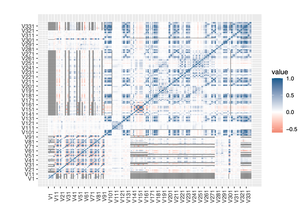
Although, there is a strong correlation beween the Vxxx features, as seen in figure 7, it is quite ambiguous to separate each of the correlations. Instead, we use dimensionality reduction techniques like Principal Component Analysis, or PCA. The results of PCA shows that, the first 16 features account for more than 99% variance in the data. Hence, we include V1~V16 in our analysis and eliminate the others.
Identity Information (id_01-id_11)
The variables id_01 to id_11 capture identity information of the transactions. Although, this is not available for all the transactions, we can analyse for patterns in available data. Additionally, we eliminate the features with more than 99% missing data.
### id_01 ~ id_11 :  Variables with more than 99% of the values as NA
missing_vars <- data.frame(Var = names(colMeans(is.na(df))),
                           missingPercent = colMeans(is.na(df))) %>%
  filter(round(missingPercent,2) >= 0.99) %>%
  pull(Var)
# id_01 ~ id_38 variables dataframevariables dataframe
id_vars_df <- select(df,names(df)[str_detect(names(df),"^id_[0-9]+")])
# Remove variables with more than 99% values missing
numeric_id_vars_df <- select(df,names(select(df,names(id_vars_df)[1:11],-all_of(missing_vars))))
# Pairwise Correlation heatmap of id_01~id11
cor(numeric_id_vars_df,
    use="pairwise.complete.obs") %>%
  melt() %>%
  dplyr::mutate(Var1=as.numeric(gsub("id_([0-9]+)","\\1",Var1)),
         Var2=as.numeric(gsub("id_([0-9]+)","\\1",Var2))) %>%
  ggplot(aes(factor(Var1),factor(Var2),fill=value)) +
  geom_tile() +
  scale_fill_gradient2(low = "#d7301f",mid="white", high = "#045a8d") +
  labs(x="",y="") +
  scale_x_discrete(labels =function(x) paste0("id_",x)) +
  scale_y_discrete(labels =function(x) paste0("id_",x))
rm(numeric_id_vars_df,id_vars_df)
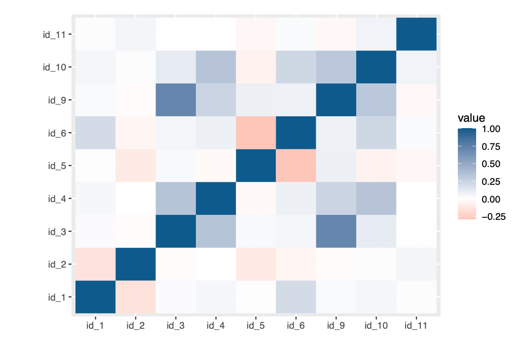
There is no strong correlation as per figure 8. Moreover, the analysis shows that, 9 variables have more than 99% of values missing. We will eliminate these from our analysis.
Categorical Variables
There are 49 categorical predictor variables in our dataset. We examine each one of the categorical variables one by one in this section.
Product Code
The ProductCD indicates the product used in each transaction. We begin our analysis, to check if any specific product is more prone to fraudulent transactions. The following code estimates the fraction of transactions and transaction amount contributed by each of the products. The boxplot for each of the products depicts the distribution of each of the individual products.
### ProductCD : product code, the product for each transaction
# Fraudulent transactions vs legitimate transactions grouped by ProductCD
df %>%
  group_by(ProductCD,isFraud) %>%
  dplyr::summarise(num_txn = n()) %>%
  data.frame() %>%
  dplyr::mutate(prop = num_txn/sum(num_txn)) %>%
  ggplot(aes(x = ProductCD,y = prop, fill = factor(isFraud))) +
  geom_bar(stat="identity",
           position=position_dodge(),
           alpha=0.7,
           color="white") +
  geom_text(aes(x = ProductCD, y = prop,
                label = paste0(round(prop * 100,2), '%')),
            position=position_dodge(0.9),
            size=2.5,vjust = -1) +
  labs(x = "Product Code",y = "% of Number of Transactions") +
  scale_y_continuous(labels = scales::percent,limits = c(0,1)) +
  scale_fill_manual("",values=c("#66c2a5","#fc8d62"),labels=c("Legitimate","Fraud")) +
  theme(legend.position = "bottom")
# Total Transaction amount of Fraudulent transactions vs legitimate transactions grouped by ProductCD
df %>%
  group_by(isFraud,ProductCD) %>%
  dplyr::summarise(Txn_amount = sum(TransactionAmt)/1000) %>%
  ggplot(aes(x = ProductCD,y = Txn_amount, fill = factor(isFraud))) +
  geom_bar(stat="identity",
           position=position_dodge(),
           alpha=0.7,
           color="white") +
  geom_text(aes(x = ProductCD, y = Txn_amount,
                label = paste0(round(Txn_amount,2),"$")),
            position=position_dodge(0.9),
            size = 2,vjust=-0.1) +
  facet_wrap(ProductCD ~.,scales = "free") +
  scale_fill_manual("",values=c("#66c2a5","#fc8d62"),labels =c("Legitimate","Fraud")) +
  labs(y="Total Transaction Amount (in Thousands)",x = "") +
  theme(legend.position = "bottom")
# Distribution of Transaction amount of Fraudulent transactions vs legitimate transactions grouped by ProductCD
df %>%
  ggplot(aes(x = ProductCD,y = TransactionAmt, fill = factor(isFraud))) +
  geom_boxplot(outlier.colour="red",
               outlier.shape=1,
               alpha=0.7) +
  labs(y="Transaction Amount") +
  ylim(0,1500) +
  coord_flip() +
  scale_fill_manual("",
                    values=c("#66c2a5","#fc8d62"),
                    labels = c("Legitimate", "Fraud")) +
  theme(legend.position = "bottom")

Although, the proportion of fraud transactions is dependant on the number of transactions in a particular product, product code is an essential feature of transaction and we therefore retain this feature for our analysis.
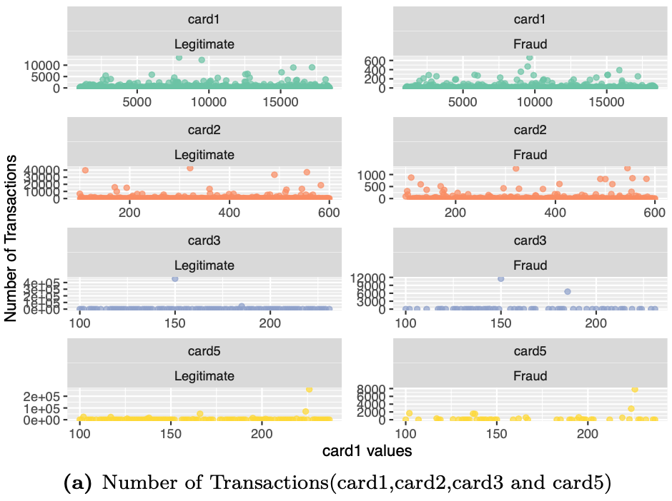
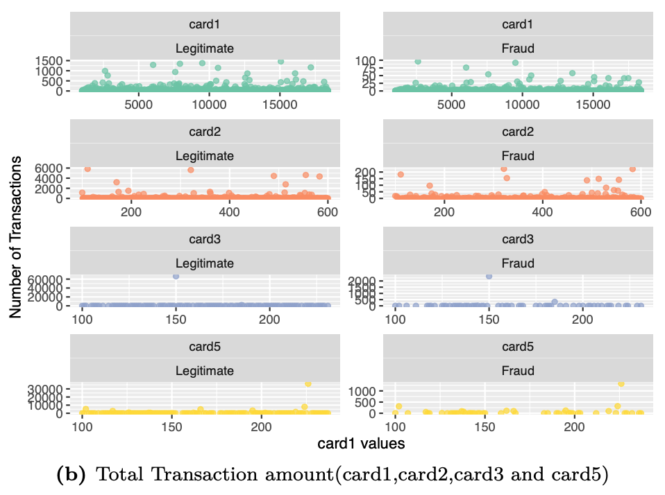
Payment Card Information
The payment card information includes 6 variables card1~card6. The information in these variable contain details such as card type, card category, issue bank, country, etc. We shall now examine an overview of these variables by the number of transactions and transaction amount in each category.
### card1 - card6 : payment card information, such as card type, card category, issue bank, country, etc.
# Visualizing  variables Card 1, Card2 and Card3 and Card5 and associated number of transactions
df %>%
  select(isFraud,card1,card2,card3,card5) %>%
  gather("Card","Values",-isFraud) %>%
  group_by(Card,isFraud,Values) %>%
  dplyr::summarise(num_txn = n()) %>%
  ggplot(aes(x = Values,y = num_txn,color=factor(Card))) +
  geom_point(alpha=0.7) +
  scale_color_manual("",values=c("#66c2a5","#fc8d62","#8da0cb","#ffd92f","#bc80bd")) +
  facet_wrap(Card ~ isFraud,
             scales = "free",
             labeller = labeller(isFraud = c("0"= "Legitimate","1" = "Fraud")),
             ncol=2) +
  labs(x ="card1 values",y="Number of Transactions") +
  theme(legend.position = "none")
# Visualizing  card1, card2, card3 and card5 values and associated transaction amount
df %>%
  select(isFraud,TransactionAmt,card1,card2,card3,card5) %>%
  gather("Card","Values",-isFraud,-TransactionAmt) %>%
  group_by(Card,isFraud,Values) %>%
  dplyr::summarise(txn_amt = sum(TransactionAmt)/1000) %>%
  ggplot(aes(x = Values,y = txn_amt,color=factor(Card))) +
  geom_point(alpha=0.7) +
  scale_color_manual("",values=c("#66c2a5","#fc8d62","#8da0cb","#ffd92f","#bc80bd")) +
  facet_wrap(Card ~ isFraud,
             scales = "free",
             labeller = labeller(isFraud = c("0"= "Legitimate","1" = "Fraud")),
             ncol=2) +
  labs(x ="card1 values",y="Number of Transactions") +
  theme(legend.position = "none")
# Visualizing variables card4 and card6
# Number of transactions for each Card type and network, grouped by transaction type(Fraudulent/legitimate)
df %>%
  dplyr::mutate(card4 = replace_columnval(card4,
                                          unique(df$card4)[!str_detect(unique(df$card4),
                                                                            "visa|master|discover|amer")],"Others"),
                card6 = replace_columnval(card6,unique(df$card6)[!str_detect(unique(df$card6),
                                    "debit|credit")],"Others")) %>%
  group_by(isFraud,card4,card6) %>%
  dplyr::summarise(num_txn = n()) %>%
  ggplot(aes(y = num_txn,x = card6, fill=factor(card6))) +
  geom_bar(stat="identity",alpha=0.8,position=position_dodge()) +
  facet_wrap(isFraud ~ card4 ,
             scales = "free",
             labeller = labeller(isFraud = c("0"= "Legitimate","1" = "Fraud"),
                                 card4 = c("Other Networks"= "Other \n Networks","american express"="Amex","discover"="Discover","mastercard"="MasterCard","visa"="Visa")),
             ncol = 5) +
  scale_fill_manual("",values=c("#66c2a5","#fc8d62","#8da0cb","#ffd92f","#bc80bd")) +
  labs(y="Number of Transactions",x = "Card Type") +
  theme(legend.position = "none",
        axis.text.x = element_text(angle = 90))
# Total transaction amount for each Card type and network, grouped by transaction type(Fraudulent/legitimate)
df %>%
  dplyr::mutate(card4 = replace_columnval(card4,
                                          unique(df$card4)[!str_detect(unique(df$card4),
                                                                       "visa|master|discover|amer")],"Others"),
                card6 = replace_columnval(card6,unique(df$card6)[!str_detect(unique(df$card6),
                                                                             "debit|credit")],"Others")) %>%
  group_by(isFraud,card4,card6) %>%
  dplyr::summarise(Txn_amount = sum(TransactionAmt)/1000) %>%
  ggplot(aes(y = Txn_amount,x = card6, fill=factor(card6))) +
  geom_bar(stat="identity",alpha=0.8) +#position=position_dodge()
  facet_wrap(isFraud ~ card4 ,
             scales = "free",
             labeller = labeller(isFraud = c("0"= "Legitimate","1" = "Fraud"),
                                 card4 = c("Other Networks"= "Other Networks","american express"="Amex","discover"="Discover","mastercard"="MasterCard","visa"="Visa")),
             ncol = 5) +
  labs(y="Transaction Amount (in Thousands)",x = "Card Type") +
  scale_fill_manual("",values=c("#66c2a5","#fc8d62","#8da0cb","#ffd92f","#bc80bd")) +
  theme(legend.position = "none",
        axis.text.x = element_text(angle = 90))
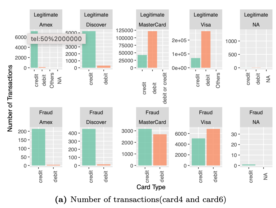
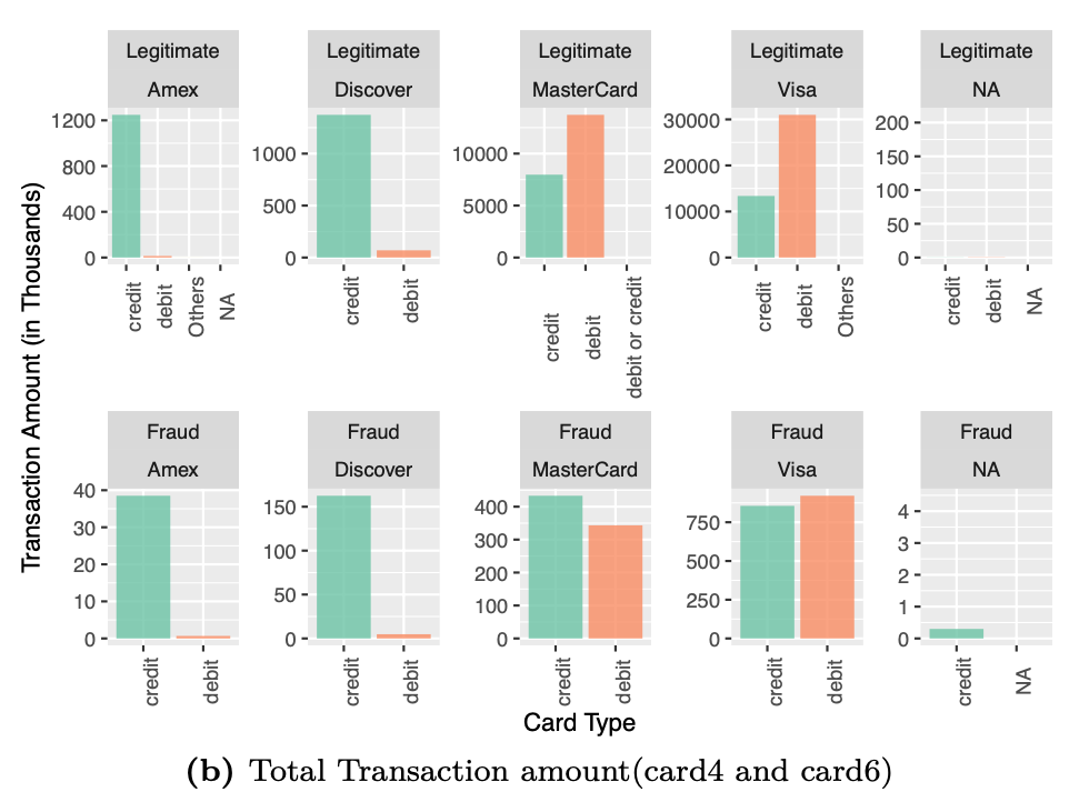
The figure shows the number of transactions and transaction amount in each of card4 and card6 categories. For example, even though the majority of legitimate transactions are on debit card in MasterCard, the number of credit card fraud transactions exceed those of debit card transations. Payment card information is quite an essential detail with respect to predicting fraud transactions. We retain all these features.
Match
We then proceed to analyze the match variables M1~M9. These features denote match, such as names on card and address, etc. The number of transactions and total amount associated with each kind of value can be viewed in the plots below.
Except for M4 variables, all other match variables are of boolean type. We will visualize both of them separately to look for patterns to identify transactions as fraud.
### M1 ~ M9 (logical) : match, such as names on card and address, etc.
# Visualizing M1~ M9 values and associated number of transactions
df %>%
  select(isFraud,M1:M3,M5:M9) %>%
  gather("Var","values",-isFraud) %>%
  group_by(Var,isFraud,values) %>%
  dplyr::summarise(num_txn = n()) %>%
  ggplot(aes(x = Var,y = num_txn,fill=factor(Var))) +
  geom_bar(stat="identity",
           alpha=0.65,
           position = position_dodge()) +
  scale_fill_brewer(type="qual",palette=3) +
  facet_wrap(values ~ isFraud,
             scales = "free",
             labeller = labeller(isFraud = c("0"= "Legitimate","1" = "Fraud")),
             ncol=2) +
  labs(x ="",y="Number of Transactions") +
  theme(legend.position = "bottom",
        axis.text.x = element_blank(),
        axis.ticks.x = element_blank())
# Visualizing M1~M9 values and associated total transaction amount
df %>%
  select(TransactionAmt,isFraud,M1:M3,M5:M9) %>%
  gather("Var","values",-TransactionAmt,-isFraud) %>%
  group_by(Var,isFraud,values) %>%
  dplyr::summarise(txn_amt = sum(TransactionAmt)/1000) %>%
  ggplot(aes(Var,y=txn_amt,fill=factor(Var))) +
  scale_fill_brewer(type="qual",palette=3) +
  geom_bar(stat="identity",
           alpha=0.65,
           position = position_dodge()) +
  facet_wrap(values ~ isFraud,
             scales = "free",
             labeller = labeller(isFraud = c("0"= "Legitimate","1" = "Fraud")),
             ncol=2) +
  labs(x="",y="Total Transaction Amount (in Thousands)") +
  theme(legend.position = "bottom")
### M4 (Character variable)
# Visualizing M4 values and associated number of transactions
df %>%
  select(isFraud,M4) %>%
  dplyr::mutate(M4 = replace(M4,is.na(M4),"(Blank)")) %>%
  group_by(isFraud,M4) %>%
  dplyr::summarise(num_txn = n()) %>%
  ggplot(aes(x = M4,y = num_txn,color = factor(isFraud),fill=factor(M4))) +
  geom_bar(stat="identity",
           position = position_dodge()) +
  scale_fill_brewer(type="qual",palette=1) +
  scale_color_manual("",values=c("#66c2a5","#fc8d62")) +
  facet_wrap(vars(isFraud),
             scales = "free",
             labeller = labeller(isFraud = c("0"= "Legitimate","1" = "Fraud")),
             ncol=2) +
  labs(x ="M4 values",y="Number of Transactions") +
  theme(legend.position = "none")
# Visualizing M4 values and associated total transaction amount
df %>%
  select(TransactionAmt,isFraud,M4) %>%
  dplyr::mutate(M4 = replace(M4,is.na(M4),"(Blank)")) %>%
  group_by(isFraud,M4) %>%
  dplyr::summarise(txn_amt = sum(TransactionAmt)/1000) %>%
  ggplot(aes(x = M4,y = txn_amt,color = factor(isFraud),fill=factor(M4))) +
  geom_bar(stat="identity",
           position = position_dodge()) +
  scale_fill_brewer(type="qual",palette=1) +
  scale_color_manual("",values=c("#66c2a5","#fc8d62")) +
  facet_wrap(vars(isFraud),
             scales = "free",
             labeller = labeller(isFraud = c("0"= "Legitimate","1" = "Fraud")),
             ncol=2) +
  labs(x ="M4 values",y="Total Transaction Amount (in Thousands)") +
  theme(legend.position = "none")
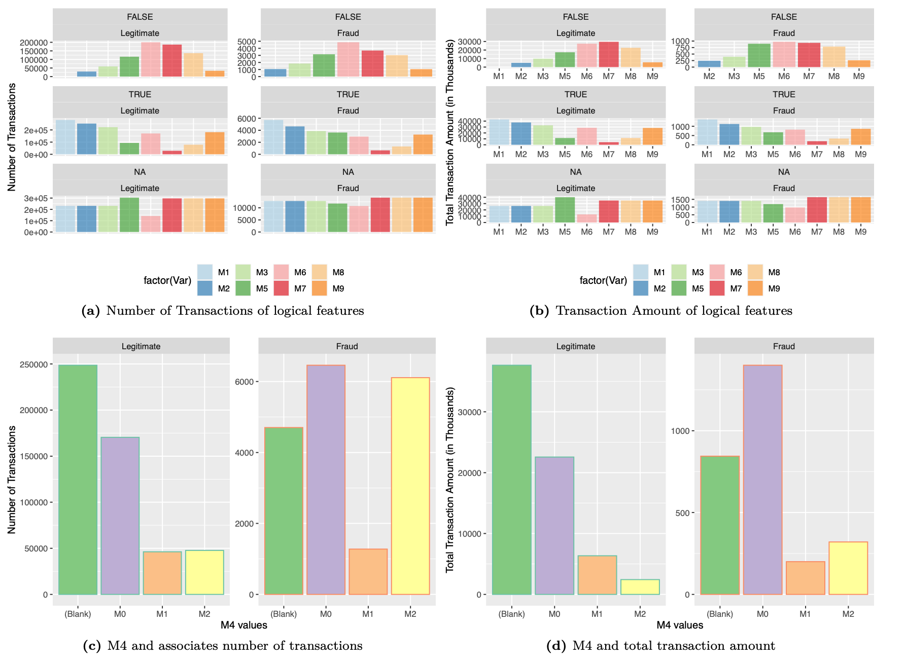
There is variance accounted by each of these features. We retain all these features for modeling.
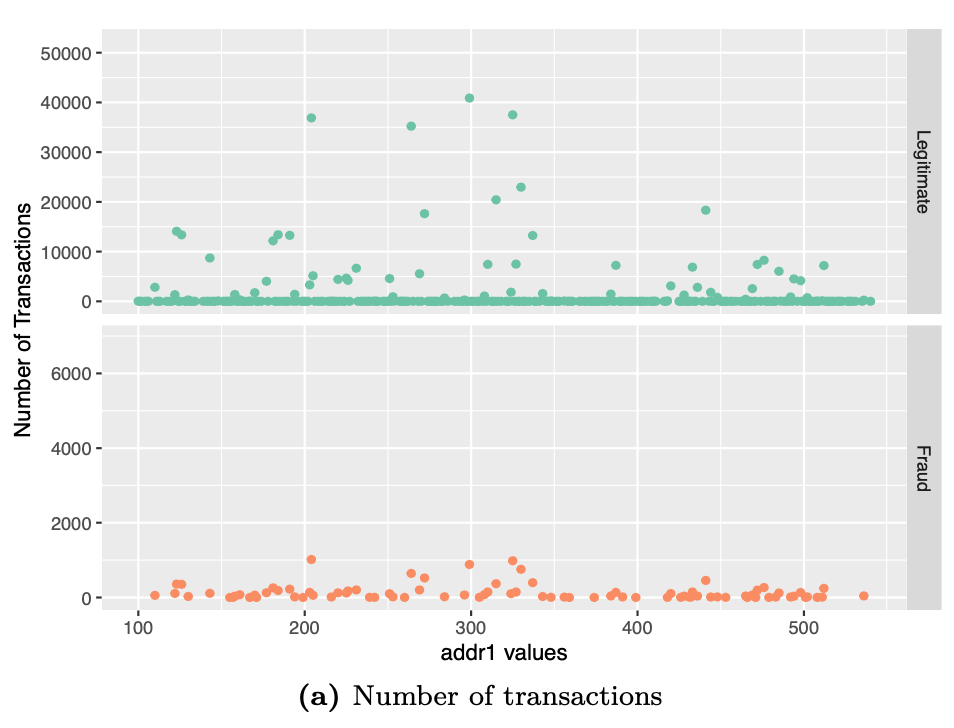
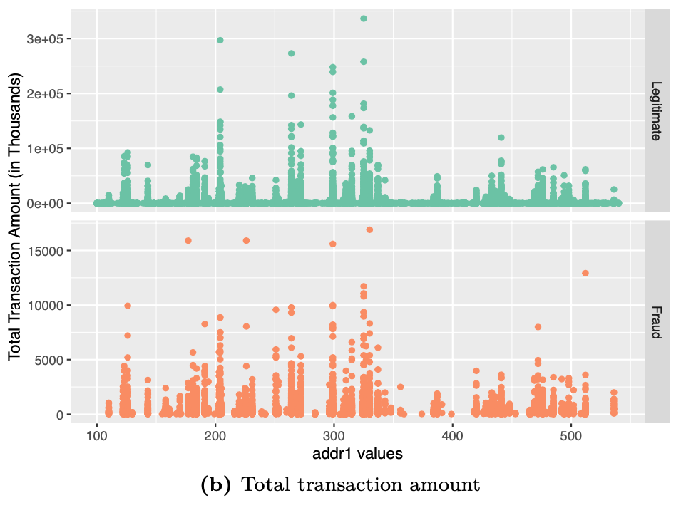
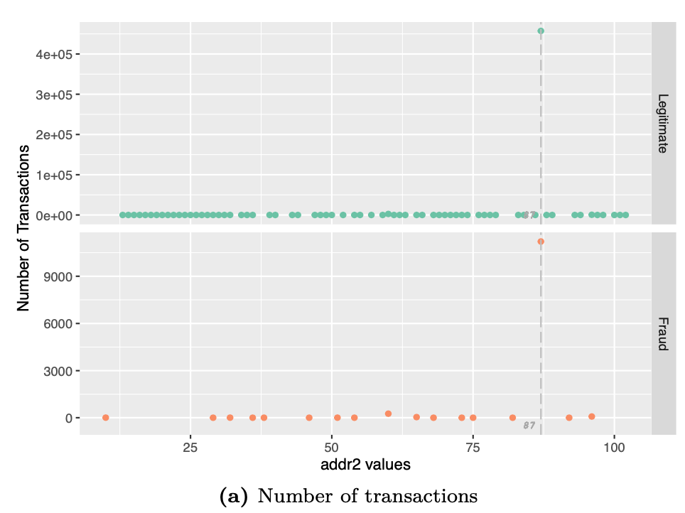
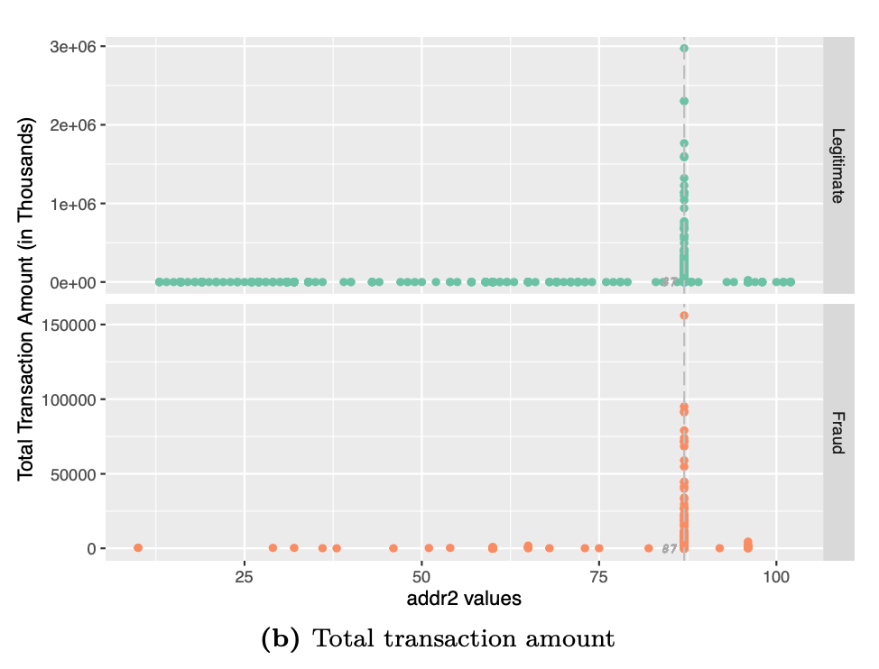
Address
The address details are given by addr1 and addr2 columns. We examine addr1 and addr2 separately to look for discernible patterns.
### addr1 and addr2 : Address
# Visualizing addr1 values and associated number of transactions
df %>%
  group_by(isFraud,addr1) %>%
  dplyr::summarise(num_txn = n()) %>%
  ggplot(aes(addr1,num_txn,color=factor(isFraud))) +
  geom_point() +
  scale_color_manual("",values=c("#66c2a5","#fc8d62")) +
  facet_grid(rows = vars(isFraud),
             scales = "free",
             labeller = labeller(isFraud = c("0"= "Legitimate","1" = "Fraud"))) +
  labs(x ="addr1 values",y="Number of Transactions") +
  theme(legend.position = "none")
# Visualizing addr1 values and associated total transaction amount
df %>%
  group_by(isFraud,TransactionAmt,addr1) %>%
  dplyr::summarise(txn_amt = sum(TransactionAmt)) %>%
  ggplot(aes(addr1,txn_amt,color=factor(isFraud))) +
  geom_point() +
  scale_color_manual("",values=c("#66c2a5","#fc8d62")) +
  facet_grid(rows = vars(isFraud),
             scales = "free",
             labeller = labeller(isFraud = c("0"= "Legitimate","1" = "Fraud"))) +
  labs(x ="addr1 values",y="Total Transaction Amount (in Thousands)") +
  theme(legend.position = "none")
# Visualizing addr2 values and associated number of transactions
df %>%
  group_by(isFraud,addr2) %>%
  dplyr::summarise(num_txn = n()) %>%
  ggplot(aes(addr2,num_txn,color=factor(isFraud))) +
  geom_point() +
  scale_color_manual("",values=c("#66c2a5","#fc8d62")) +
  geom_vline(xintercept=87,linetype = "longdash",color="grey") +
  geom_text(aes(87,y=-500,label=87,hjust=1.5),
            size=2.5,family="Courier", fontface="italic",color="darkgrey") +
  facet_grid(rows = vars(isFraud),
             scales = "free",
             labeller = labeller(isFraud = c("0"= "Legitimate","1" = "Fraud"))) +
  labs(x ="addr2 values",y="Number of Transactions") +
  theme(legend.position = "none")
# Visualizing addr2 values and associated total transaction amount
df %>%
  group_by(isFraud,TransactionAmt,addr2) %>%
  dplyr::summarise(txn_amt = sum(TransactionAmt)) %>%
  ggplot(aes(addr2,txn_amt,color=factor(isFraud))) +
  geom_point() +
  scale_color_manual("",values=c("#66c2a5","#fc8d62")) +
  geom_vline(xintercept=87,linetype = "longdash",color="grey") +
  geom_text(aes(87,y=-500,label=87,hjust=1.5),
            size=2.5,family="Courier", fontface="italic",color="darkgrey") +
  facet_grid(rows = vars(isFraud),
             scales = "free",
             labeller = labeller(isFraud = c("0"= "Legitimate","1" = "Fraud"))) +
  labs(x ="addr2 values",y="Total Transaction Amount (in Thousands)") +
  theme(legend.position = "none")
Purchaser email domain
The purchaser email domain is given by P_emaildomain. We merge the domains appropriately to ease our analysis with domains. We merge all microsoft, yahoo, icloud, aol, gmail and .net(Networking) domains separately and categorize all other domains as “Others”.
### P_emaildomain: purchaser email domain
# Visualizing purchaser email domain of approximately 99% of the transactions.
df %>%
  dplyr::mutate(P_emaildomain = replace_columnval(P_emaildomain,c("live","outlook","hotmail","msn"),"Microsoft"),
                # Replaces 8 Yahoo domains
                P_emaildomain = replace_columnval(P_emaildomain,c("yahoo","ymail"),"Yahoo"),
                # Replaces 3 icloud domains
                P_emaildomain = replace_columnval(P_emaildomain,c("me.com","mac.com","icloud.com"),"iCloud"),
                # Replaces 2 AOL domains
                P_emaildomain = replace_columnval(P_emaildomain,c("aol","aim"),"AOL"),
                P_emaildomain = replace_columnval(P_emaildomain,c("gmail.com","gmail"),"Gmail"),
                P_emaildomain = replace_columnval(P_emaildomain,c(".net"),"NetworkingDomains"),
                P_emaildomain = replace_columnval(P_emaildomain,unique(df$P_emaildomain)[!str_detect(unique(df$P_emaildomain),
                                                                                                          "Gmail|Yahoo|Networking|Microsoft|AOL|iCloud")]
                                                  ,"Others")) %>%
  dplyr::mutate(P_emaildomain = replace(P_emaildomain,is.na(P_emaildomain),"Unknown")) %>%
  group_by(isFraud,P_emaildomain) %>%
  dplyr::summarise(num_txn = n()) %>%
  ggplot(aes(reorder(P_emaildomain,num_txn),num_txn,fill=factor(isFraud))) +
  geom_bar(stat="identity",position=position_dodge()) +
  scale_fill_manual("",values=c("#66c2a5","#fc8d62")) +
  facet_wrap(vars(isFraud),
             scales = "free",
             labeller = labeller(isFraud = c("0"= "Legitimate","1" = "Fraud"))) +
  coord_flip() +
  labs(x ="Purchaser email domain",y="Number of transactions") +
  theme(legend.position = "none",
        axis.text.x = element_text(angle = 90))
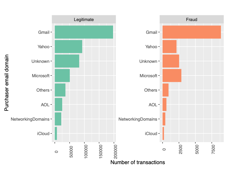
The figure shows the number of legitimate transactions for yahoo exceeds all others except gmail. But, the number of fraud transactions from microsoft exceeds that of yahoo. There are some patterns which need more analysis and hence we retain the variable in our model.
Recepient email domain
The recepient email domain is given by R_emaildomain. Similar to the purchaser email domain, we merge the domains appropriately to ease our analysis with domains. We merge all microsoft, yahoo, icloud, aol, gmail and .net(Networking) domains separately and categorize all other domains as “Others”.
### R_emaildomain : recipient email domain
# Visualizing recipient email domain of approximately 99% of the transactions.
df %>%
  dplyr::mutate(R_emaildomain = replace_columnval(R_emaildomain,c("live","outlook","hotmail","msn"),"Microsoft"),
                R_emaildomain = replace_columnval(R_emaildomain,c("yahoo","ymail"),"Yahoo"),
                R_emaildomain = replace_columnval(R_emaildomain,c("me.com","mac.com","icloud.com"),"iCloud"),
                R_emaildomain = replace_columnval(R_emaildomain,c("aol","aim"),"AOL"),
                R_emaildomain = replace_columnval(R_emaildomain,c("gmail.com","gmail"),"Gmail"),
                R_emaildomain = replace_columnval(R_emaildomain,c(".net"),"NetworkingDomains"),
                R_emaildomain =
                  replace_columnval(R_emaildomain,
                                    unique(df$R_emaildomain)[!str_detect(unique(df$R_emaildomain),
                                                                              "Gmail|Yahoo|Networking|Microsoft|AOL|iCloud")],"Others")) %>%
  dplyr::mutate(R_emaildomain = replace(R_emaildomain,is.na(R_emaildomain),"Unknown")) %>%
  group_by(isFraud,R_emaildomain) %>%
  dplyr::summarise(num_txn = n()) %>%
  ggplot(aes(reorder(R_emaildomain,num_txn),num_txn,fill=factor(isFraud))) +
  geom_bar(stat="identity",position=position_dodge()) +
  scale_fill_manual("",values=c("#66c2a5","#fc8d62")) +
  facet_wrap(vars(isFraud),
             scales = "free",
             labeller = labeller(isFraud = c("0"= "Legitimate","1" = "Fraud"))) +
  coord_flip() +
  labs(x ="Recepient email domain",y="Number of transactions") +
  theme(legend.position = "none",
        axis.text.x = element_text(angle = 90))
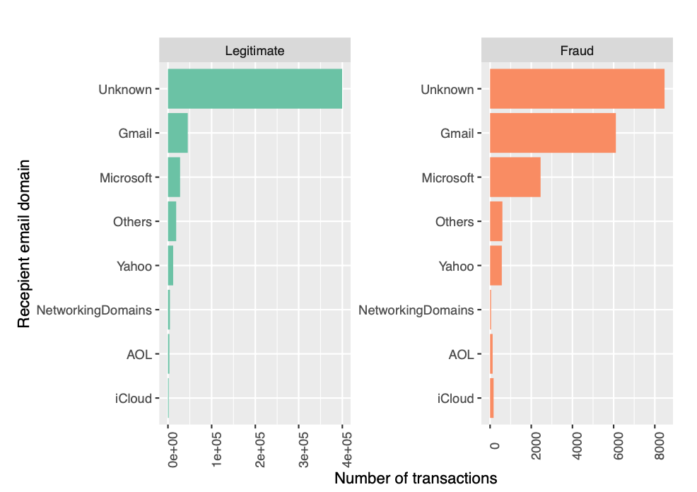
We see similar patters with recipient email domain as well. Even though number of legitimate transactions are higher in aol when compared to icloud, the latter has higher fraud transactions.
Device Type
The variable DeviceType gives the type of device used for the online transaction. We shall examine the number of transactions in each category.
### Device Type : type of device used for transaction (mobile/desktop/Unknown)
df %>%
  dplyr::mutate(DeviceType = replace(DeviceType,is.na(DeviceType),"Unknown")) %>%
  group_by(isFraud,DeviceType) %>%
  dplyr::summarise(num_txn = n()) %>%
  ggplot(aes(y = num_txn,x = DeviceType, fill=factor(isFraud))) +
  geom_bar(stat="identity",alpha=0.8,position=position_dodge()) +
  facet_wrap(vars(isFraud),
             scales = "free",
             labeller = labeller(isFraud = c("0"= "Legitimate","1" = "Fraud"))) +
  scale_fill_manual("",values=c("#66c2a5","#fc8d62")) +
  labs(y="Number of Transactions",x = "Device Type") +
  theme(legend.position = "none")

Although the number of legitimate transactions using desktop exceeds that of mobile, the number of fraud transactions using mobile is slightly higher than that of desktop. We shall retain the variable for inclusion in our model.
Device Info
The device information of the device on which the transaction was made can is available in the DeviceInfo column. We analyse the device information of devices that have more than 100 transactions.
### Device Info
df %>%
  select(DeviceType,DeviceInfo,isFraud) %>%
  dplyr::mutate(DeviceInfo = replace_columnval(DeviceInfo,c("SM","SAMSUNG","samsung"),"Samsung"),
                DeviceInfo = replace_columnval(DeviceInfo,c("HTC"),"HTC"),
                DeviceInfo = replace_columnval(DeviceInfo,c("Moto","Motorola","MOTOROLA","XT1635"),"Motorola"),
                DeviceInfo = replace_columnval(DeviceInfo,c("HUAWEI","Huawei","hi6210"),"Huawei"),
                DeviceInfo = replace_columnval(DeviceInfo,c("LG"),"LG"),
                DeviceInfo = replace(DeviceInfo,is.na(DeviceInfo),"Unknown")) %>%
  dplyr::mutate(DeviceType = replace(DeviceType,is.na(DeviceType),"Unknown")) %>%
  group_by(DeviceType,DeviceInfo,isFraud) %>%
  dplyr::summarise(num=n()) %>%
  arrange(-num) %>%
  filter(num>100) %>%
  ggplot(aes(y = num,x = DeviceInfo, fill=factor(isFraud))) +
  geom_bar(stat="identity",alpha=0.8,position=position_dodge()) +
  facet_wrap(isFraud~DeviceType,
             scales = "free",
             labeller = labeller(isFraud = c("0"= "Legitimate","1" = "Fraud"),
                                 DeviceType = c("desktop"="Desktop","mobile"="Mobile","Unknown"="Unknown"))) +
  scale_fill_manual("",values=c("#66c2a5","#fc8d62","#8da0cb")) +
  labs(y="Number of Transactions",x = "Device Information") +
  theme(legend.position = "none",
        axis.text.x = element_text(angle = 90))
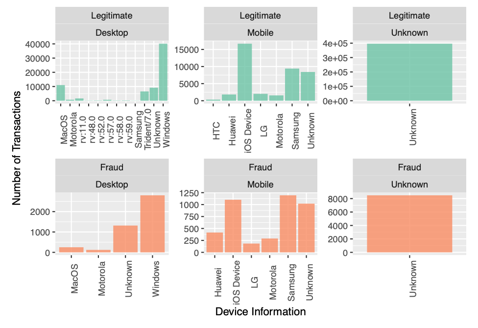
There are visible patterns in the visualization above and hence we use this variable in our model.
Identity Information (id_12~id_38)
The identity information available in id12~id38 contain information regarding the device where transaction was made. For example : id_30 gives the OS version, id_31 gives the browser version, id_33 gives the resolution of the device to name a few. We retain all these variables, since they give further details of the transaction.
Data Preprocessing
This stage involves various data preprocessing tasks like handling missing data, encoding categorical data as numerical and imputing missing values.
#################################################
##### Feature Selection & Imputing missing data
#################################################
# 434 Features in original dataset
##### Initial Feature Selection by EDA
eliminated_features <- c(c_vars_drop,d_vars_missingvalues,vxxx_vars_drop,missing_vars)
rm(c_vars_drop,d_vars_missingvalues,vxxx_vars_drop,missing_vars)
##### Feature Engineering : Label Encoding and One-hot encoding
# This function encodes the dataset and imputes necessary missing values
feature_engg_fraud_det <- function(temp){
  # Eliminated 350 variables after EDA; Remaining 84 variables
  numeric_df <- select(temp,-all_of(eliminated_features)) %>% select_if(is.numeric)  #  Numeric vectors
  char_df <- select(temp,-all_of(eliminated_features)) %>% select_if(is.character)   #  Character vectors
  logical_df <- select(temp,-all_of(eliminated_features)) %>% select_if(is.logical) # 12 Logical vectors

# Merging email domains, card values and imputing missing categorical values
char_df <- char_df %>%
              dplyr::mutate(card6 = replace_columnval(card6,
                                                      unique(char_df$card6)[!str_detect(unique(char_df$card6),
                                                                            "debit|credit")],"Others")) %>%
              dplyr::mutate(card4 = replace_columnval(card4,
                                                      unique(char_df$card4)[!str_detect(unique(char_df$card4),
                                                                                        "visa|master|discover|amer")],
                            "Others")) %>%
              dplyr::mutate(P_emaildomain = replace_columnval(P_emaildomain,
                                                              c("live","outlook","hotmail","msn"),
                                                              "Microsoft"),
                           # Replaces Yahoo domains
                            P_emaildomain = replace_columnval(P_emaildomain,
                                                  c("yahoo","ymail"),
                                                  "Yahoo"),
                           # Replaces icloud domains
                           P_emaildomain = replace_columnval(P_emaildomain,c("me.com","mac.com","icloud.com"),"iCloud"),
                           # Replaces AOL domains
                           P_emaildomain = replace_columnval(P_emaildomain,
                                                             c("aol","aim"),
                                                             "AOL"),
                           P_emaildomain = replace_columnval(P_emaildomain,
                                                             c("gmail.com","gmail"),
                                                             "Gmail"),
                           P_emaildomain = replace_columnval(P_emaildomain,
                                                             c(".net"),
                                                             "NetworkingDomains"),
                           P_emaildomain = replace_columnval(P_emaildomain,
                                                             unique(char_df$P_emaildomain)[!str_detect(unique(char_df$P_emaildomain),
                                                                                                       "Gmail|Yahoo|Networking|Microsoft|AOL|iCloud")]
                                                             ,"Others")) %>%
             dplyr::mutate(R_emaildomain = replace_columnval(R_emaildomain,
                                                             c("live","outlook","hotmail","msn"),
                                                             "Microsoft"),
                R_emaildomain = replace_columnval(R_emaildomain,
                                                  c("yahoo","ymail"),
                                                  "Yahoo"),
                R_emaildomain = replace_columnval(R_emaildomain,
                                                  c("me.com","mac.com","icloud.com"),
                                                  "iCloud"),
                R_emaildomain = replace_columnval(R_emaildomain,
                                                  c("aol","aim"),
                                                  "AOL"),
                R_emaildomain = replace_columnval(R_emaildomain,
                                                  c("gmail.com","gmail"),
                                                  "Gmail"),
                R_emaildomain = replace_columnval(R_emaildomain,
                                                  c(".net"),
                                                  "NetworkingDomains"),
                R_emaildomain = replace_columnval(R_emaildomain,
                                                  unique(char_df$R_emaildomain)[!str_detect(unique(char_df$R_emaildomain),
                                                                                                          "Gmail|Yahoo|Networking|Microsoft|AOL|iCloud")]
                                                  ,"Others")) %>%
             dplyr::mutate(DeviceType =  replace(DeviceType,is.na(DeviceType),"Unknown"),
                           DeviceInfo =  replace(DeviceInfo,is.na(DeviceInfo),"Unknown"),
                           card4 = replace(card4,is.na(card4),"Unknown"),
                           card6 = replace(card6,is.na(card6),"Unknown"),
                           P_emaildomain = replace(P_emaildomain,is.na(P_emaildomain),"Unknown"),
                           R_emaildomain = replace(R_emaildomain,is.na(R_emaildomain),"Unknown"),
                           M4 =  replace(M4,is.na(M4),"Unknown"),
                           id_12 = replace(id_12,is.na(id_12),"Unknown"),
                           id_15 = replace(id_15,is.na(id_15),"Unknown"),
                           id_16 = replace(id_16,is.na(id_16),"Unknown"),
                           id_28 = replace(id_28,is.na(id_28),"Unknown"),
                           id_29 = replace(id_29,is.na(id_29),"Unknown"),
                           id_30 = replace(id_30,is.na(id_30),"Unknown"),
                           id_31 = replace(id_31,is.na(id_31),"Unknown"),
                           id_34 = replace(id_34,is.na(id_34),"Unknown")) %>%
  # Dropping resolution column
  select(-id_33)
  # Binding columns of the dataset :  106 variables
  temp_df <-
    # 5 character vectors encoded as 28 one-hot encoded variables
    cbind(as.data.frame(sapply(names(char_df)[str_detect(names(char_df),
                                                         "emaildomain|card|Product")],
                               function(x) one_hot_encoding(char_df,x))),
          # 11 character variables encoded with label encoding to 11 variables
          as.data.frame(sapply(names(char_df)[!str_detect(names(char_df),
                                                          "emaildomain|card|Product")],
                               function(x) label_encoding(char_df,x))),
          # 12 logical vectors encoded as 12 numeric encoding of logical variables
          as.data.frame(sapply(names(logical_df),
                               function(x) as.numeric(logical_df[[x]]))),
          # 55 numeric variables
          numeric_df)

  # Imputing numerical NA as -999
  temp_df <- temp_df %>% dplyr::mutate_if(is.numeric, list(~replace_na(., -999)))

  return (temp_df)
}
We then create a 90/10 train-test split of the df dataset for our model evaluation purposes. The model is created and trained in the train set and tested in the test set. This is called the prototyping phase that revolves around model selection, which requires measuring the AUC of plausible candidate models. When we are satisfied with the selected model type and hyperparameters, the last step of the prototyping phase is to train a new model on the entire df dataset set using the best hyperparameters found. The model is then validated on data we had put aside, the validation set. This gives us an estimate of the generalization error.i.e how well our model generalizes to new data.
#### Create train set, test set (Imbalanced)
df <- feature_engg_fraud_det(df)
set.seed(1234, sample.kind="Rounding")
# Create train set and test set
test_index <- createDataPartition(y = df$isFraud, times = 1 ,p=0.1, list = FALSE)
imbal_train_set <- df[!row.names(df) %in% test_index,]
imbal_test_set <- df[row.names(df) %in% test_index,]
# Remove unwanted variables
rm(test_index)
Dealing with Imbalanced Classes
We previously discussed the effects of imbalanced data on our machine learning algorithms. Algorithms tend to overfit the data and classify all the transactions as legitimate and fail to discern patterns in the fraudulent transactions. However, there are methods to mitigate this and balance the data before feeding it to the models. We can achieve balanced classes by downsampling the majority class or oversampling the minority class. Although, with random undersampling method there is a loss in information of the non-fraud transactions, it is optimal method with regards to computational efficiency. Oversampling the minority class can be achieved using Synthetic Minority Oversampling Technique, or SMOTE. With our current dataset, deploying SMOTE to balance the dataset needs excessive computational resources. Therefore, we proceed with random downsampling. In this method, the random samples are chosen from majority class and all minority class transactions in the dataset is retained.
Classification Models
Bagged Classification and Regression Trees (Bagged CART)
The first modeling technique chosen for the fraud detection dataset is the bagged classification and regression trees, or bagged CART. The bagging refers to the bootstrap aggregation of CART. Bagging is a very powerful ensemble method used for minimizing the variance in algorithms with high variance. One of the algorithms with high variance is the decision tree or CART. We use the method treebag that implements bagging technique from the ipred package. We use nbagg to control the number of bootstrap replications. Although, bagged CART is efficient and powerful, they are less desired if the data is correlated. Additionally, it tends to become computationally intense with an increase in the number of bootstrap samples. Therefore, we proceed to examine better techniques to overcome the observed drawbacks of bagged CART.
Random Forest
Random forests build an ensemble of deep independent trees to improve the predictive performance. Random forests are an improvement over bagged decision trees. The fundamental principle behind random forests are same as that of decision trees. They help to minimize the tree correlation by randomly picking the bootstrapped samples. The algorithm performs split-variable randomization where each time a split is to be performed and the search for the split variable is controlled by the mtry parameter. The default value of mtry is $\sqrt{p}$ for classification model.
eXtreme Gradient Boosting(XGBOOST)
Gradient Boosting Techniques are extremely popular machine learning algorithms and have proven successful across various domains. Gradient Boosting Machines(GBMs) build an ensemble of shallow trees in sequence, with each tree learning from the previous and are highly efficient, flexible and portable.
Results
This section presents the code and results of the models discussed in the previous section. We will measure AUC for each of the models discussed above. The trainControl function is used to set the parameters to control how models are created. The models we chose in the previous section will be used along with these parameters. We will use repeated cross validation technique with 5-fold cross validation and the sampling technique used is the random down sampling technique. The classProbs is set to TRUE to enable the models to compute class probabilities, so that, AUC can be estimated.
# Computational control parameters for train function
fitControl = trainControl(method = "repeatedcv", # Repeated Cross validation
                          number = 5,  #  controls the number of folds in K-fold cross-validation
                          #repeats = 5, # Repeats K-fold cross-validation
                          verboseIter = FALSE, # A logical for printing a training log.
                          returnData = FALSE, #  A logical for saving the data into a slot called trainingData
                          allowParallel = TRUE, # Use a parallel processing if available
                          sampling = "down", # Balancing imbalanced dataset using random downsampling
                          classProbs = TRUE, #  class probabilities be computed for classification models
                          summaryFunction = twoClassSummary) # a function to computed alternate performance summaries.
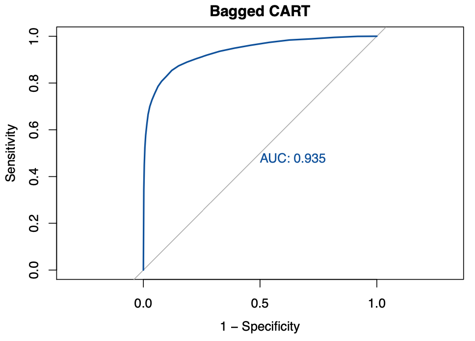
Bagged CART
The following code accomplishes the bagged CART with a default of 25 bagged trees for faster computation.
#### Model 1 : Bagged CART
# Setting seed for reproducibility
set.seed(231, sample.kind="Rounding")
# Train the model to find the best tune for bagged CART;
# Used default nbagg=25 for faster computation
fit.bagcart <-
  train(
    make.names(isFraud)~.,
    data = imbal_train_set,
    trControl = fitControl,
    method = "treebag",
    metric ="ROC",
    tree_method = "hist",
    nthread = 2,
    verbose = TRUE)
# Predictions on imbalanced test set
pred.bagcart <- predict(fit.bagcart,
                           imbal_test_set %>% select(-isFraud),
                           type="prob")
# ROC for Bagged CART
roctreebag_down <-  roc(imbal_test_set$isFraud,
                        factor(pred.bagcart$X1, ordered = TRUE),
                        plot=TRUE,
                        smooth = FALSE,
                        print.auc=TRUE,
                        col = "#08519c",
                        legacy.axes=TRUE,
                        main="Bagged CART",
                        levels = c("0", "1"))
roctreebag_down
auc_results <- tibble(method = "Bagged CART",
                      AUC = roctreebag_down$auc)
auc_results %>% knitr::kable()
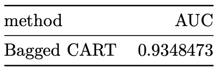
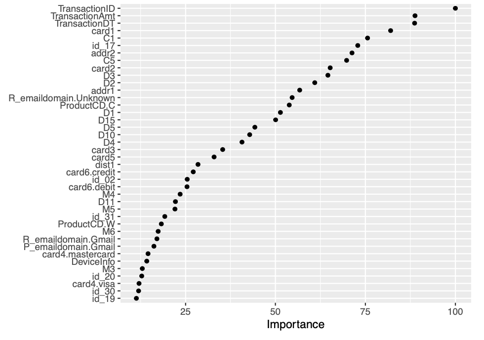
The AUC achieved by the bagged CART model corresponds to 0.93485. We then proceed to construct a variable importance plot (VIP) of the top 40 features in the bagged CART model.
vip::vip(fit.bagcart, num_features = 40, geom = "point")
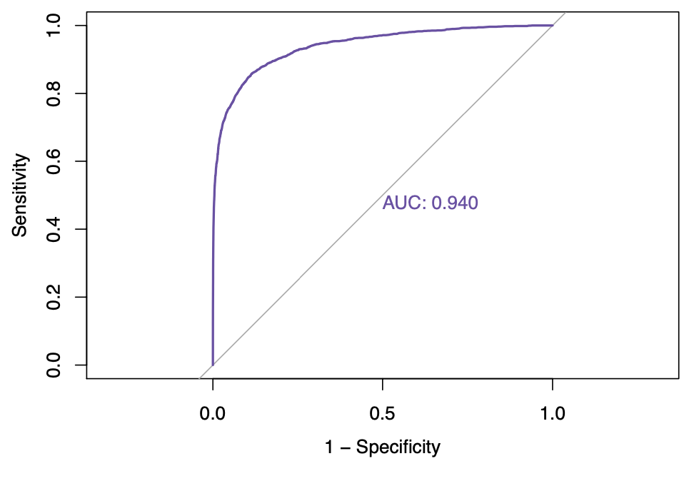
Random Forest
In this section, we implement random forest algorithm for our fraud detection data. The mtry hyperparameter that controls split-variable randomization feature of random forests has been set to square root of the number of variables in our model.
# Model 2 : Random Forest
# mtry (The number of features to consider at any given split) for Classification models
mtry = floor(sqrt(ncol(imbal_train_set)))
# Creating hyperparameter grid search for Random Forest
rfgrid <- expand.grid(.mtry=mtry)
# Setting seed for reproducibility
set.seed(112, sample.kind="Rounding")
# Train the model to find the best tune for Random Forest
fit.randomforest = train(
  make.names(isFraud)~.,
  data = imbal_train_set,
  trControl = fitControl,
  tuneGrid = rfgrid,
  method = "rf",
  tree_method = "hist",
  metric ="ROC",
  verbose = TRUE)
# Predict with imbalanced test set
pred.rf <- predict(fit.randomforest,
                        imbal_test_set %>% select(-isFraud),
                        type = "prob")
# Generating ROC for the Random Forest model
rf_down <- roc(imbal_test_set$isFraud,
                factor(pred.rf$X1,ordered=TRUE),
                plot=TRUE,
                print.auc=TRUE,
                col = "#6a51a3",
                legacy.axes=TRUE,
                levels = c("0", "1"))
rf_down
auc_results <-
  rbind(auc_results,tibble(method = "Random Forest",
                            AUC =rf_down$auc))
auc_results %>% knitr::kable()
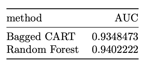
We observe that, we saw an improvement of AUC with the random forest algorithm. The AUC achieved by the bagged CART model corresponds to 0.94022. We then proceed to construct a variable importance plot (VIP) of the top 40 features in the bagged CART model.
vip::vip(fit.randomforest, num_features = 40, geom = "point")
eXtreme Gradient Boosting(XGBOOST)
The following code accomplishes the XGBOOST with best tune parameters, obtained after a grid search on a hyperparameter grid of values. Boosting iterations has been restricted to 500 for optimal computational efficiency. The other parameters like maximum tree depth, learning rate/shrinkage, minimum loss reduction(gamma), subsample ratio of columns, maxiumum sum of instance weight and subsample percentage has been estimated after training the model with a hyperparameter grid of various values.
# Model 3 : XGBOOST (eXtreme Gradient Boosting)
# Creating hyperparameter grid search for XGBOOST Hyperparameters with faster learning rate of 0.1
xgbGrid = expand.grid(nrounds = 500,   # Boosting Iterations : Number of trees or rounds
                      max_depth = 15,  # c(5, 10, 15), # Max Tree Depth : Controls the depth of the individual trees
                      eta = 0.1,       # Learning rate/ Shrinkage
                      gamma = 1,       # c(1, 2, 3), # Minimum Loss Reduction : Pseudo-regularization hyperparameter known as a Lagrangian multiplier and controls the complexity of a given tree.
                      colsample_bytree = 1, # c(0.4, 0.7, 1.0), # Subsample Ratio of Columns
                      min_child_weight = 0.5, # c(0.5, 1, 1.5), # Minimum Sum of Instance Weight
                      subsample = 0.7 ) # Subsample Percentage

# Setting seed for reproducibility
set.seed(212, sample.kind="Rounding")
# Train the model to find the best tune for XGBOOST
fit.xgboost = train(
  make.names(isFraud)~.,
  data = imbal_train_set,
  trControl = fitControl,
  tuneGrid = xgbGrid,
  method = "xgbTree",
  tree_method = "hist",
  metric ="ROC",
  verbose = TRUE)
# Predict with imbalanced test set
pred.xgboost <- predict(fit.xgboost,
                           imbal_test_set %>% select(-isFraud),
                           type = "prob")
# Generating ROC for the XGBOOST model
xgb_down <- roc(imbal_test_set$isFraud,
                factor(pred.xgboost$X1,ordered=TRUE),
                plot=TRUE,
                print.auc=TRUE,
                col = "#993404",
                legacy.axes=TRUE,
                levels = c("0", "1"))
xgb_down
auc_results <-
  rbind(auc_results,tibble(method = "XGBOOST",
                            AUC =xgb_down$auc))
auc_results %>% knitr::kable()
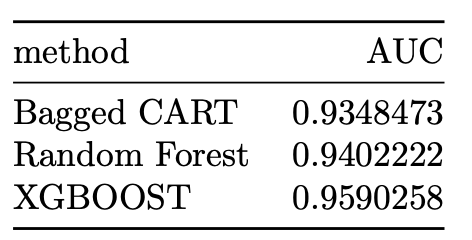
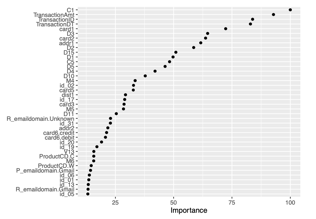
We see further improvement in AUC with the XGBOOST algorithm. The AUC achieved by the XGBOOST model corresponds to 0.95903. We then proceed to construct a variable importance plot (VIP) of the top 40 features in the XGBOOST model.
vip::vip(fit.xgboost, num_features = 40, geom = "point")
Final Validation
Once we are confident about our final model, we measure AUC on the validation set, to estimate the generalization performance. This is the last step of prototyping phase where we will train a new model on the entire set using the best hyperparameters found. In the case of fraud detection dataset, the finalized model is XGBOOST model. Now, we train the complete model with the df dataset and estimate the AUC on validation set.
### AUC of finalized model(XGBOOST) with the validation set
# Set random seed
set.seed(1234, sample.kind = "Rounding")
# Training the full model with the best tuning hyperparameters
fxgb = train(
  make.names(isFraud)~.,
  data = df,
  trControl = fitControl,
  tuneGrid = xgbGrid,
  method = "xgbTree",
  tree_method = "hist",
  metric ="ROC",
  verbose = TRUE)
# Predictions on the validation set
pred.xgboost <- predict(fxgb,
                           feature_engg_fraud_det(validation_x),
                           type = "prob")
# Generating ROC Curve for XGBOOST on validation dataset
rocxgb_down_validation <- roc(validation_y$isFraud,
                              factor(pred.xgboost$X1,ordered=TRUE),
                              plot=TRUE,
                              print.auc=TRUE,
                              col = "#006d2c", # green
                              legacy.axes=TRUE,
                              main="AUC with XGBOOST(Validation Set)",
                              levels = c("0", "1"))
rocxgb_down_validation
auc_results <-
  rbind(auc_results,tibble(method = "XGBOOST (Validation Set)",
                            AUC =rocxgb_down_validation$auc))
auc_results %>% knitr::kable()
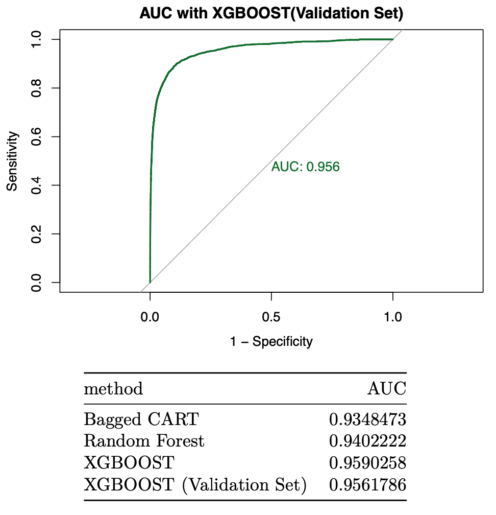
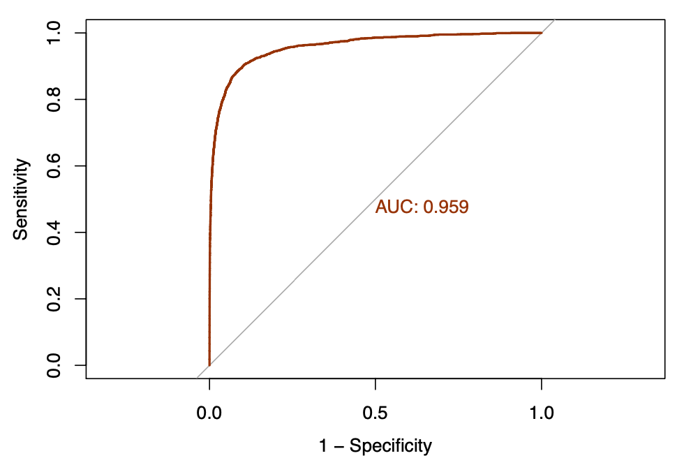
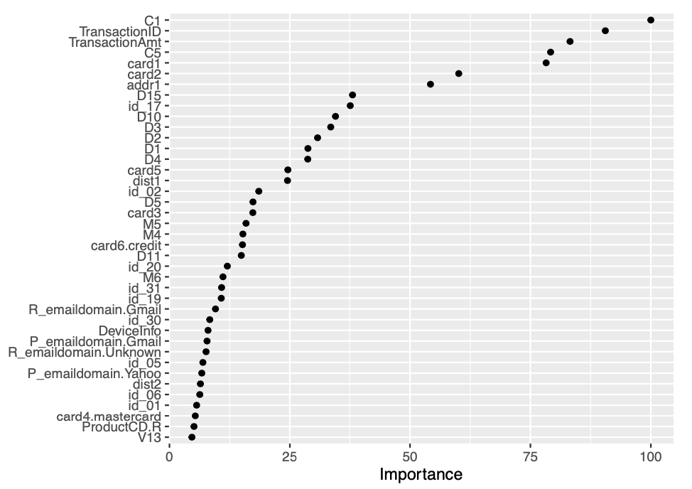
The AUC achieved by the XGBOOST on validation set corresponds to 0.95618. We then proceed to construct a variable importance plot (VIP) of the top 40 features in the XGBOOST model on validation set.
vip::vip(fxgb, num_features = 40, geom = "point")

Conclusion
The performance of each of the algorithms can be significantly improved with higher number of iterations in case of bagged CART and number of boosting iterations in case of XGBOOST. Regardless of the the computational intensity of the algorithms discussed above, it is vital to note that gradient boosting machines are one of the most powerful ensemble algorithms offering excellent accuracy. Although, we discussed XGBOOST(one of the most popular GBMs), there are better alternatives for this as well. One of them, is the CatBoost that uses efficient methods for encoding categorical features and is expected to perform well in situations with frequent changes in data. Yet another alternative for traditional GBMs is, the LightGBM. It focuses on leaf-wise tree growth versus the level-wise tree growth of the traditional GBMs. It offers key advantages of faster training speed, lower memory usage among others.
Thanks for reading! If you want to get in touch with me or leave me any feedback, feel free to reach me on my email. You can find the complete script in my github repository.
References
(1) Baesens, Bart, Véronique van Vlasselaer, and Wouter Verbeke. Fraud Analytics Using Descriptive, Predictive, and Social Network Techniques : Guide to Data Science for Fraud Detection / Bart Baesens, Veronique Van Vlasselaer, Wouter Verbeke. 1st edition. Hoboken, New Jersey: John Wiley & Sons, 2015.
(2) Alice Zheng, Amanda Casari. Feature Engineering for Machine Learning: Principles and Techniques for Data Scientists.O’Reilly Media, Inc.April 2018.
(3) Alice Zheng. Evaluating Machine Learning Models.O’Reilly Media, Inc.September 2015
(4) Matt Harrison. Machine Learning Pocket Reference. O’Reilly Media, Inc.August 2019