Loan Amortization

Introduction
This article is part of a series about financial modeling using python/vba/R where I cover some of the prominent financial models useful for analysts. In this article we will explore loan amortization using Excel and Python. If you follow along for both, you’ll understand the concept at a deeper level, but feel free to navigate directly to the Excel or Python sections however you please.
So, what does it mean when a loan is amortized?
Amortization, derived from a Latin word admortire, which means “to kill”, simply refers to paying off an amount owed over time by making planned, incremental payments of principal and interest.
In the following section, we will talk about some key terms on amortization before jumping onto the code and building a amortization schedule.
Amortization Schedule
An amortization schedule is a complete table of periodic loan payments, showing the amount of principal and the amount of interest that comprise each payment until the loan is paid off at the end of its term.
Components of a Amortization Schedule in a Financial Model
- Loan amount : Original or expected balance for your mortgage/loan.
- Term in years : The number of years over which you will repay this loan.
- Interest rate : Annual fixed interest rate for this loan.
- Payment per period : Also called as Equated Monthly Installment (EMI), includes principal payment and interest payment (PI). While each periodic - payment is the same amount early in the schedule, the majority of each payment is interest; later in the schedule, the majority of each payment covers the loan’s principal.
- Total interest : Total of all interest paid over the full term of the mortgage. This total interest amount assumes that there are no prepayments of principal.
- Total payments : Total of all monthly payments over the full term of the mortgage. This total payment amount assumes that there are no prepayments of principal.
Next, lets discuss the design and layout of the amortization calculator that we are going to build in following sections. We shall build our excel amortization model with three sections: loan information/summary grid, loan EMI data table and an amortization schedule.
Loan Amortization using Microsoft Excel
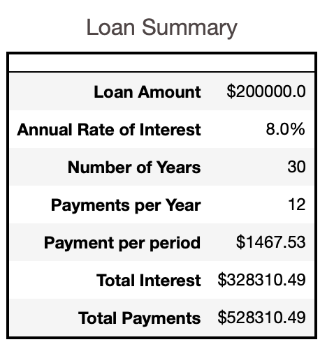
We begin initializing our input to the amortization calculator, such as, the annual interest rate, amortization period, payments per year, and the loan amount (principal). Let’s consider a 30-year loan of 200,000 USD with monthly payments at an 8% annual rate of interest. This should require a monthly payment of $1,467.53 to fully amortize the loan.

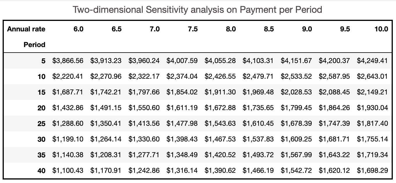
The loan EMI data table is a table that does a sensitivity analysis on the loan information provided in the summary. This paragraph elaborates on the implementation of two-dimensional excel data tables to perform sensitivity analysis on the payment per period/EMI with loan term and the annual interest rate. Figure 2 illustrates the sensitivity analysis on the payment per period. We see that, the upper left-hand corner of our data table contains, the formula as a reference to the payment per period(available in the loan summary section). We now use the Data Table command. We fill in both the Row input cell (indicating the cell that contains loan term in the loan summary) and the Column input cell (indicating the cell that contains annual interest rate in the loan summary).

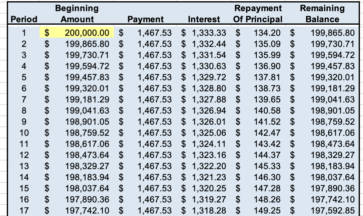
We then proceed with generating the loan amortization schedule. Figure 3 depicts a portion of amortization schedule for the user input from loan summary section. We will be using IF statements in the amortization table so that changes in the “Number of Years” and/or “Payments per Year” input variables will be correctly incorporated into the cells. We use the excel functions PMT, IPMT, and PPMT to compute the “Payment” and “Interest” and “Repayment of Principal” column entries, respectively.

This concludes the implementation of loan amortization using microsoft excel. To modify any of the cells or edit the worksheet, you can fork my github repository or get a copy of the entire spreadsheet from the embedded workbook below.
Loan Amortization using Python
To begin, we shall recreate a layout similar to that of excel spreadsheet. For obvious reasons, we will use the pandas library to achieve such a layout since this project demands us to create data frames. The first step is to load the required libraries and then we will create user defined functions for generating the loan summary, sensitivity analysis and the amortization schedule.
# Libraries needed
import numpy as np
import numpy_financial as npf
import pandas as pd
from IPython.display import display, HTML
We will then create some helper functions to validate the input variables to our model. The following code is useful for validating the principal, annual rate of interest, loan term and the number of payments per year.
#Input Validation for Principal, annual rate , loan term and no of payments
class InputValidation:
    """
    This class validates the inputs (Principal, annual rate, term in years and number of payments per year)
    Principal(principal) : Validates if input Loan amount is a positive integer
    Annual Rate(annual_interest_rate) : Validates if the Annual rate is >0
    Term in Years(per): Validates if term is a positive finite integer
    No of Payments(nper):Validates if nper is a positive finite integer
    """
    def __init__(self,inputvar):
        self.inputvar = inputvar

    #Method for checking if the input variable is a positive integer value (Eg. Principal)
    def check_positive_integer(self):
        while True:
            try:
                tempvar = float(input(f"\nPlease Enter a positive integer value for {self.inputvar}:"))
                if tempvar.is_integer() and tempvar>0:
                    break
                else:
                    print(f"\n{self.inputvar} should be a positive integer value!")
            except:
                print(f"\n{self.inputvar} is not a number!")

        return tempvar

    #Method for checking if the input variable is a positive value (Eg. Annual interest rate) --
    def check_positive_float(self):
        while True:
            try:
                tempvar = float(input(f"\nPlease Enter a positive integer value for {self.inputvar}:"))
                if tempvar>0 and tempvar < 100:
                    break
                else:
                    print(f"\n{self.inputvar} should be a positive value greater than 0 and less than 100!")
            except:
                print("\nNot a valid Option!! Try again..")
        return tempvar

    #Method for checking if the input variable is a finite term (Eg.Loan term and No. of payments per year)
    def finiteterm_check(self):
        while True:
            try:
                tempvar = float(input(f"\nPlease Enter a positive integer value for {self.inputvar}:"))
                if tempvar.is_integer() and tempvar>0 and tempvar<100:
                    break
                else:
                    print(f"\n{self.inputvar} should be a positive integer value less than 100!")
            except:
                print(f"\n{self.inputvar} is not a number!")

        return tempvar
Next, we will display the summary and loan information that is input by the user. We will use the function generate_summary to generate an overview of the loan summary table. The code below implements the user defined function to generate the loan summary.
def generate_summary(principal,initial_rate,per,nper):
    """
    This function generates summary for amortization schedule
    """
    mysum = generate_payment_schedule(principal,initial_rate,per,nper)
    total_interest = mysum["Interest Expense"].sum().round(2)
    pmt = -npf.pmt(initial_rate/nper,per*nper,principal)
    total=total_interest+principal
    mymatrix = pd.DataFrame(['$'+str(pmt.round(2)),'$'+str(total_interest.round(2)),'$'+str(total.round(2))],
                            columns=[""],
                            index=["Payment per period","Total Interest","Total Payments"])

    return mymatrix
We will then create a user defined function generate_matrix for generating the payment per period for various rates and terms to perform a sensitivity analysis on the payment per period. We have used a general range for loan term from 5 to 40 years with a step size of 5 years. The following code generates a data table for various values of loan term and annual rate of interest.
# Function to generate matrix of various term vs rate of interest
def generate_matrix(principal,paymentfreq,initial_rate,ratestep,period,periodstep):
    """
    This function generates the payment matrix at various rates and terms
    """
    # Generates a matrix of 6 x 9 matrix with payments at various
    # Declaring Row iterator
    termrows = [i for i in range(5,45,periodstep)]

    # Declaring Column Iterator
    #ratecolumn = [(round(j*100,3)) for j in np.arange(initial_rate,initial_rate+ 4.5/100,ratestep)]
    ratecolumn = [(round(j*100,3)) for j in np.arange(initial_rate - 2/100,initial_rate,ratestep)]  +\
    [(round(j*100,3)) for j in np.arange(initial_rate+ratestep,initial_rate+ 2.25/100,ratestep)]

    # Naming axis and index
    mymatrix = pd.DataFrame(columns =ratecolumn ,index=termrows).rename_axis('Annual rate',axis=1)
    mymatrix['Period']=termrows
    mymatrix.set_index('Period',inplace=True)

    # Generating Payment matrix for generated list of period and rates
    for i in termrows:
        for j in ratecolumn:
            mymatrix.at[i,j] = -npf.pmt(float(j/100)/paymentfreq,i*paymentfreq,principal)

    return (mymatrix)
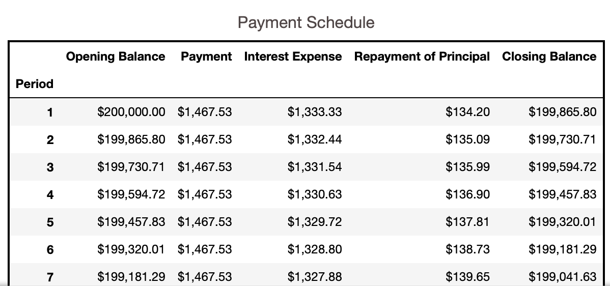
The next task is to create an amortization schedule with period, opening balance, payment per period(EMI), interest expense, repayment of principal and the closing balance. Similar to previously created tables, we will use a user defined function to generate this table as well. The following code implements function generate_payment_schedule to create an amortization schedule.
def generate_payment_schedule(principal,annual_interest_rate,per,nper):
    """
    This function generates the amortization schedule
    """
    # Declaration of Variables
    periodic_interest_rate = annual_interest_rate/nper
    no_of_payments = nper*per

    # Defining the Structure of DataFrame
    columnnames =['Period','Opening Balance','Payment','Interest Expense','Repayment of Principal','Closing Balance']

    # Filling Static Columns & Index
    period=[i for i in range(1,no_of_payments+1)]

    # Formatting the DataFrame
    # pd.options.display.float_format = '${:,.2f}'.format

    # Initialization of the DataFrame
    mymatrix = pd.DataFrame(columns =columnnames,index=period)

    # Calculations
    mymatrix.at[1,'Opening Balance']=principal
    mymatrix['Period']=period
    mymatrix.set_index('Period',inplace=True)
    mymatrix['Payment']=-npf.pmt(periodic_interest_rate,no_of_payments,principal)
    mymatrix['Interest Expense']=-npf.ipmt(periodic_interest_rate,mymatrix.index, no_of_payments,principal)
    mymatrix['Repayment of Principal']= -npf.ppmt(periodic_interest_rate,mymatrix.index,no_of_payments,principal)


    #Calculation of dynamic part of Amortization Schedule
    for i in period:
        if i>1:
            mymatrix['Closing Balance']= mymatrix['Opening Balance']-mymatrix['Repayment of Principal']
            mymatrix.at[i,'Opening Balance']=mymatrix.at[i-1,'Closing Balance']
        if mymatrix.at[i,'Opening Balance']-mymatrix.at[i,'Repayment of Principal']<0.1:
            mymatrix.at[i,'Closing Balance']=0


    mymatrix.at[1,'Opening Balance']=principal
    return (mymatrix)
This is then followed by the main part of the code which will accept a user input and generate all the data tables discussed above using the functions created. This is achieved by the code below.
def amortization_table():
    """ Calculate the loan amortization schedule given the loan details

     Arguments:
        annual_interest_rate: The annual interest rate for this loan
        per: Number of years for the loan
        nper: Number of payments in a year
        principal: Amount borrowed

    Returns:
        matrix : Returns a 6 x 9 matrix of payments at various rates and term
        schedule: Amortization schedule as a pandas dataframe
        summary: Pandas dataframe that summarizes the payoff information
    """
    # Taking User Input
    principalval = InputValidation("Principal")
    principal= principalval.check_positive_integer()

    rateval = InputValidation("Annual Interest Rate")
    annual_interest_rate=rateval.check_positive_float()/100

    pervalidation = InputValidation("Loan Term in years")
    per = int(pervalidation.finiteterm_check())

    npervalidation = InputValidation("No of Payments per year")
    nper = int(npervalidation.finiteterm_check())

    # Input information on the loan
    loan_df = pd.DataFrame(['$'+ str(principal),str(annual_interest_rate*100)+'%',per,nper],
                            columns=[""],
                            index=["Loan Amount","Annual Rate of Interest","Number of Years","Payments per Year"])


    # Payment at various rates vs term
    matrix = generate_matrix(principal,nper,annual_interest_rate,0.005,per,5)

    # Amortization Schedule
    schedule = generate_payment_schedule(principal,annual_interest_rate,per,nper)
    summary= generate_summary(principal,annual_interest_rate,per,nper)


    display(pd.concat([loan_df, summary], axis=0).style.set_caption("Loan Summary").set_table_styles([
                                      {'selector' : '',
                                       'props' : [('background-color','white'),
                                                  ('border','2px solid black')]},
                                      {'selector': 'caption',
                                       'props': [('color', '#4f4646'),
                                                 ('font-size', '16px'),
                                                 ('text-align', 'center')]}]))

    display(matrix.style.set_caption("Two-dimensional Sensitivity analysis on Payment per Period").set_table_styles([
                            {'selector' : '',
                            'props' : [('background-color','white'),
                                       ('border','2px solid black')]},
                            {'selector': 'caption',
                            'props': [('color', '#4f4646'),
                                      ('font-size', '16px'),
                                      ('text-align', 'center')]}]).format('${:,.2f}'))

    print("\n \033[1m Based on the information you entered, your payment is {} for {} years with a rate of {}%\033[1m".\
          format(summary.at["Payment per period",""],per,annual_interest_rate*100))

    display(schedule.style.set_caption("Payment Schedule").set_table_styles([
                            {'selector' : '',
                            'props' : [('background-color','white'),
                                       ('border','2px solid black')]},
                            {'selector': 'caption',
                            'props': [('color', '#4f4646'),
                                      ('font-size', '16px'),
                                      ('text-align', 'center')]}]).format('${:,.2f}'))


The above snapshots gives an idea of how our main function, amortization_table takes user input. Figure 5 illustrates the summary/loan information.


Figure 6 displays the data table with two-dimensional sensitivity analysis on the payment per period and Figure 7 presents the amortization schedule for the corresponding user input.

In this article, we implemented loan amortization using microsoft excel and pandas. Although both approaches are quite easy to implement, code written in python can be reused for similar projects and is more efficient. To modify any part of the code, you can fork my github repository or download this workbook by clicking on this link.
Thanks for reading! If you want to get in touch with me or leave me any feedback, feel free to reach me on my email.
References
(1) Benninga, Simon (April 2014). Financial Modeling. Cambridge, MA: MIT Press. ISBN: 9780262027281.
(2) Ross, S. A., R. W. Westerfield, and J. Jaffe. 2010. Corporate Finance, 9th ed. McGraw-Hill.