Movie Recommender system

Introduction
The evolution of e-commerce and online streaming platforms has largely grown over the past several years. Early setbacks to more widespread adoption of these services, namely delivery costs in case of online retailers and bandwidth availability, especially with the video streaming platforms, have largely faded. Now many retailers are altering their online value propositions simply because it allows them to cast a much larger net. For consumers around the globe, and across various consumer groups, online channels have become the most crucial shopping resources with millions of products and titles available compared to the physical store with only a few alternatives available.
However, one of the major factors affecting the profits of online retailers and content streaming services is the problem to reduce the confusing plethora of options posed to consumers, when navigating their websites. One of the key features of these online retailers and streaming platforms is the personalized product recommendations. Product suggestions to customers based on the products they’ve already bought, as well as on the viewing activity can improve their shopping experience and get more sales. This challenge motivates the need for recommender systems.
A recommender system analyzes data, on both products and users, to make item suggestions to a given user, indexed by u, or predict how that user would rate an item, indexed by i. Recommender system strategies broadly fit into one of the two categories: content-based filtering and collaborative filtering. A content-based filtering technique analyzes the past choices of a user and constructs profiles based on the user actions alone to build a preference profile, instead of pairing users with the products that similar users liked.
On the other hand, collaborative filtering systems analyze interactions or similarity between users and items. Its distinct because it looks at the behavior of multiple customers cross-referencing their purchase histories with each other. Good personalized recommendations enhances the user experience, thereby improving customer satisfaction and loyalty. This technique is generally more accurate than content filtering. In this project, we will utilize both strategies for building our own recommender system.
Movielens Dataset
The data used in this analysis is from the MovieLens 10M set, containing 10000054 ratings and 95580 tags applied to 10681 movies by 71567 users of the online movie recommender service MovieLens. The data is made available by GroupLens, a research group in the Department of Computer Science and Engineering at the University of Minnesota.
Loss Functions
Machine learning models are evaluated by means of a loss function. The loss function measures the difference between the predictions and the actual outcome. There are various factors involved in choosing a loss function for specific problem, such as, type of machine learning algorithm chosen, ease of calculating the derivatives, and to some degree, the percentage of outliers in the data set.
The most common loss functions for recommender systems are mean absolute error (MAE) and root-mean-square error (RMSE). One important quality of MAE is that it does not give any bias to extreme values in error terms and it will weigh those equally to the other predictions. In short, MAE is robust to outliers. On the contrary, RMSE disproportionately penalizes large errors, and is well suited for error terms that follow a normal distribution.
\[MAE = \frac {1}{N} \sum_{i=1}^{N}{|\hat{y_i} - y_i|}\]Mean Absolute Error
Mean Absolute Error (MAE) is a loss function used for regression models. MAE is the sum of absolute differences between our target and predicted variables.
The MAE is given by the formula,
where $N$ is the number of observations, $\hat{y_i}$ is the predicted value and $y_i$ is the actual value.
\[RMSE = \sqrt{\frac {1}{N} \sum_{u,i}{(\hat{y_i} - y_i)^2}}\]Root Mean Squared Error
In machine learning, root-mean-square error(RMSE) is a quantifiable way to check how a model’s fitted values stack up against actual values.
The RMSE is the typical metric to evaluate recommendation systems, and is defined by the formula:
where $N$ is the number of observations, $\hat{y_i}$ is the predicted value and $y_i$ is the actual value.
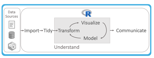
Data Analytics Workflow
Evidently, the first step in building a recommender system involves framing the problem and getting the data, well known as Data Ingestion. Then, we choose an appropriate performance metric to rightly assess our models. These metrics are also called loss functions. This is followed by data exploration and data visualization tasks which is collectively called as Exploratory Data Analysis(EDA). This is followed by various data preparation tasks depending on the type of model we are trying to build. Once this is completed, the next step is generally termed as the prototyping phase, where we train and test various candidate models and select the best model using model selection. The main task of prototyping phase is to select the model. However, there are various other tasks involved in this stage from feature selection to designing the model and training the data. The candidate models are then evaluated (Model Evaluation) based on the loss function selected and the loss function is further optimized by hyperparameter tuning. Once we are satisfied with our prototype model, the same is deployed in production to put it through further testing on live data.
In the case of movielens dataset, we consider the validation dataset as the new/unseen dataset for final validation of the chosen model.
Data Ingestion
In this stage, we download the data and prepare the dataset to be used in the analysis. The dataset is split into two datasets: mlens and validation with 90% and 10% of the original dataset respectively. We take the validation set and put it off to the side, pretending that we have never seen it before.
##########################################################
# Create mlens set, validation set (final hold-out test set)
##########################################################

# Note: this process could take a couple of minutes

if(!require(tidyverse)) install.packages("tidyverse", repos = "http://cran.us.r-project.org")
if(!require(caret)) install.packages("caret", repos = "http://cran.us.r-project.org")
if(!require(data.table)) install.packages("data.table", repos = "http://cran.us.r-project.org")
if(!require(lubridate)) install.packages("lubridate", repos = "http://cran.us.r-project.org")

library(tidyverse)
library(caret)
library(data.table)
library(lubridate)

# MovieLens 10M dataset:
# https://grouplens.org/datasets/movielens/10m/
# http://files.grouplens.org/datasets/movielens/ml-10m.zip

dl <- tempfile()
download.file("http://files.grouplens.org/datasets/movielens/ml-10m.zip", dl)

ratings <- fread(text = gsub("::", "\t", readLines(unzip(dl, "ml-10M100K/ratings.dat"))),
                 col.names = c("userId", "movieId", "rating", "timestamp"))

movies <- str_split_fixed(readLines(unzip(dl, "ml-10M100K/movies.dat")), "\\::", 3)
colnames(movies) <- c("movieId", "title", "genres")

# if using R 4.0 or later:
movies <- as.data.frame(movies) %>% mutate(movieId = as.numeric(movieId),
                                           title = as.character(title),
                                           genres = as.character(genres))

movielens <- left_join(ratings, movies, by = "movieId")

# Validation set will be 10% of MovieLens data
set.seed(1, sample.kind="Rounding") # if using R 3.5 or earlier, use `set.seed(1)`
test_index <- createDataPartition(y = movielens$rating, times = 1, p = 0.1, list = FALSE)
mlens <- movielens[-test_index,]
temp <- movielens[test_index,]

# Make sure userId and movieId in validation set are also in mlens set
validation <- temp %>%
  semi_join(mlens, by = "movieId") %>%
  semi_join(mlens, by = "userId")

# Add rows removed from validation set back into mlens set
removed <- anti_join(temp, validation)

mlens <- rbind(mlens, removed)

rm(dl, ratings, movies, test_index, temp, movielens, removed
Helper Functions
In this section, we will create the helper functions needed for this dataset for analysis and performance evaluation of models. The following code creates necessary helper functions for this project.
# This function creates one-hot encoded columns of a selected column
one_hot_encoding <- function(df,colname,delim){
  conv_list <- df[[colname]] %>%
    paste(sep="",collapse=delim)

  # Get the list of possible values category can have
  possible_val <- unique(strsplit(conv_list,"\\|")[[1]])
  temp_df <- cbind(df,sapply(possible_val, function(g) {
    as.numeric(str_detect(df[[colname]], g))
  })
  )
  colnames(temp_df) <- c(names(df), possible_val)
  return(temp_df)
}

### Loss functions
# This function calculates the Root Mean Squared Error (RMSE)
RMSE <- function(true_ratings, predicted_ratings){
  sqrt(mean((true_ratings - predicted_ratings)^2))
}

# This function calculates the Mean Absolute Error (MAE)
MAE <- function(true_ratings, predicted_ratings){
  mean(abs(true_ratings - predicted_ratings))
}
Exploratory Data Analysis
Data ingestion is followed by data exploration where we intend to gain some insights about the dataset we just loaded. We study each attribute and its characteristics like name, type, percentage of missing values, outliers, type of distribution and many others. The subsequent tasks include studying correlations between the attributes and identifying the promising transformations if needed. Data visualization is quite an important tool for accomplishing these tasks. We document all these intuitions thus obtained by summarizing and visualizing the dataset, aiding the understanding of the project. We begin our data exploration, with the structure of the dataset.
## Classes 'data.table' and 'data.frame':   9000055 obs. of  6 variables:
##  $ userId   : int  1 1 1 1 1 1 ...
##  $ movieId  : num  122 185 292 316 329 355 ...
##  $ rating   : num  5 5 5 5 5 5 ...
##  $ timestamp: int  838985046 838983525 838983421 838983392 838983392 838984474 ...
##  $ title    : chr  "Boomerang (1992)" "Net, The (1995)" ...
##  $ genres   : chr  "Comedy|Romance" "Action|Crime|Thriller" ...
##  - attr(*, ".internal.selfref")=<externalptr>
## data frame with 0 columns and 0 rows
With an initial glance of the dataset, we observe that movie information is available in movieId and title columns; user information is available in userId column, timestamp is measured in seconds with “1970-01-01 UTC” as origin; rating column is our target variable; Each movie rating has been categorized into one or more genres which is available in genres column. Each observation maps to a user ‘u’ rating a movie ‘i’.
# dataset dimensions
dim(mlens)
## [1] 9000055 6
# Counts the number of NAs in each column of the dataset
colSums(is.na(mlens))
##    userId   movieId    rating timestamp     title    genres
##         0         0         0         0         0         0
There is no missing data in this dataset. We continue our data exploration with an overview of our mlens dataset, and then proceed to visualize distribution of the variables and check for any possible outliers.
The first 6 rows of the dataset, mlens
userId	movieId	rating	timestamp	title	genres
1	122	5	838985046	Boomerang (1992)	Comedy|Romance
1	185	5	838983525	Net, The (1995)	Action|Crime|Thriller
1	292	5	838983421	Outbreak (1995)	Action|Drama|Sci-Fi|Thriller
1	316	5	838983392	Stargate (1994)	Action|Adventure|Sci-Fi
1	329	5	838983392	Star Trek: Generations (1994)	Action|Adventure|Drama|Sci-Fi
1	355	5	838984474	Flintstones, The (1994)	Children|Comedy|Fantasy
We observe that, it is in tidy format. i.e. each row matches up with a single observation and variables are available as columns. We can now begin analyzing each one of the variables. Also, to better analyze the variables, we will consider one-hot encoding of the genres data, so that, each individual genre is represented as a separate feature. The following code accomplishes one-hot encoding of genres column in the mlens dataset.
# Creates a dataset with encoded genres column of mlens
encoded_mlens <- one_hot_encoding(mlens,"genres","|")
The first 6 rows of the dataset with one-hot encoded genres column
genres	                      Comedy	Romance	Action	Crime	Thriller Drama	Sci-Fi	Adventure
Comedy|Romance	                1	1	0	0	0	0	0	0
Action|Crime|Thriller	        0	0	1	1	1	0	0	0
Action|Drama|Sci-Fi|Thriller	0	0	1	0	1	1	1	0
Action|Adventure|Sci-Fi	        0	0	1	0	0	0	1	1
Action|Adventure|Drama|Sci-Fi 	0	0	1	0	0	1	1	1
Children|Comedy|Fantasy	        1	0	0	0	0	0	0	0
Rating
We begin our analysis with the Rating column. Rating column is the dependent variable that we are going to predict using our recommender system.
# Rating Distribution
mlens %>%
  group_by(rating) %>%
  summarise(num_rating = n()) %>%
  ggplot(aes(rating,num_rating/1000)) +
  geom_bar(stat="identity") +
  xlab("Rating") +
  ylab("Number of ratings (in thousands)") +
  theme(plot.title = element_text(hjust = 0.5,face="italic"))
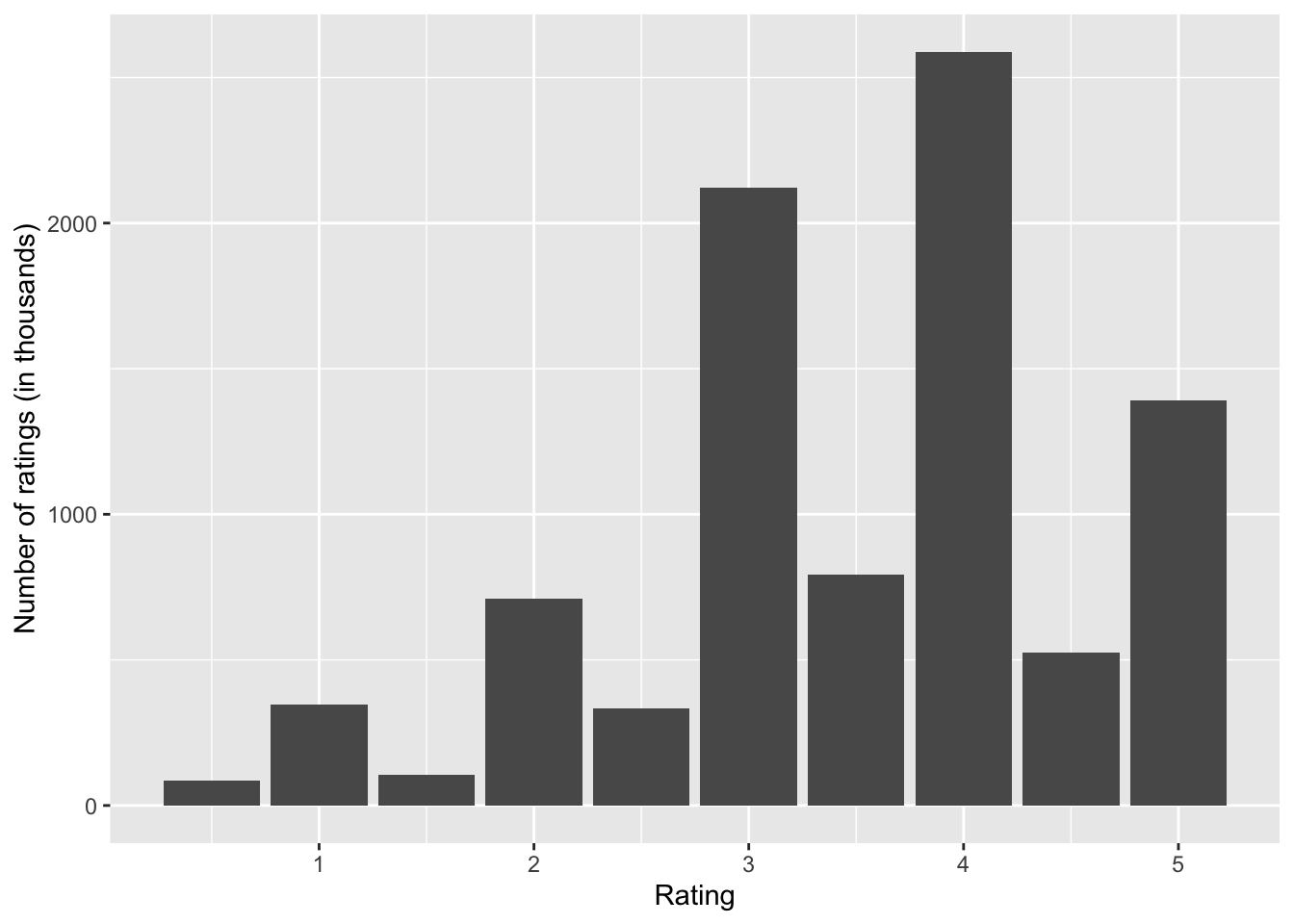
Figure 2 shows that, the users can choose a rating value between 0.5 and 5.0. In addition, it is evident from the plot that, it is less common for users to rate movies with half-star ratings.
Movies
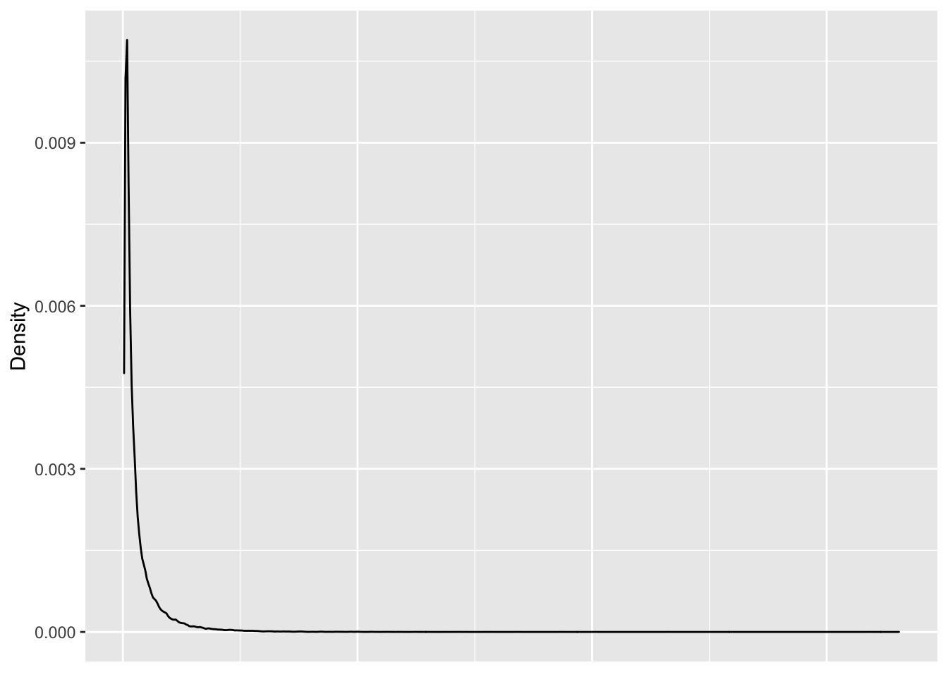
Movie information is available with two variables: movieId and title. Let’s start analyzing the variable movies, by computing the number of distinct movies in the dataset and then proceed to analyze the distribution. We visualize the distribution of movie ratings using a density plot. We understand that, the distribution is highly skewed, but it’s hard to extract further information from this plot. Additionally, if we choose histogram, we need to choose appropriate number of bins for accomodating all the data in the plot. To overcome these issues, a normalized Empirical Cumulative Distribution Function (ECDF) plot is opted, where we can gain meaningful insights without having to choose number of bins or lose clarity of data as a whole.
## [1] 10677
There are 10677 distinct movies in this dataset.
# Density plot of distribution of ratings grouped by movieId
mlens %>%
  group_by(movieId) %>%
  summarise(num_rating = n())  %>%
  ggplot(aes(num_rating)) +
  geom_density() +
  ylab("Density") +
  theme(plot.title = element_text(hjust = 0.5,face="italic"),
        axis.title.x = element_blank(),
        axis.text.x = element_blank(),
        axis.ticks.x = element_blank())
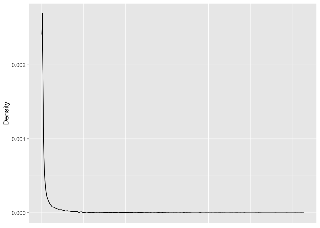
The density plot in Figure 2 depicts the distribution of user ratings grouped by user. The distribution is highly skewed, with some movies having exceedingly large number of ratings, whereas more number of movies have small number of ratings.
# Normalized ecdf of the number of ratings per movie
mlens %>%
  group_by(movieId) %>%
  summarise(num_rating = n()) %>%
  ggplot(aes(x = num_rating)) +
  stat_ecdf(geom = "step",
            size = 0.75,
            pad = FALSE) +
  theme_minimal() +
  coord_cartesian(clip = "off") +
  geom_vline(xintercept = 1000, colour = "darkgrey",alpha=0.5,linetype="dashed") +
  geom_text(aes(1000, 0, label=1000,vjust=1.5),
            size=3,family="Courier", fontface="italic",color="darkgrey") +
  geom_hline(yintercept = 0.80, colour = "darkgrey",alpha=0.5,linetype="dashed") +
  geom_text(aes(0, 0.8, label=0.8,hjust=-1),
            size=3,family="Courier", fontface="italic",color="darkgrey") +
  geom_hline(yintercept = 0.99, colour = "darkgrey",alpha=0.5,linetype="dashed") +
  geom_text(aes(0, 0.99, label=0.99,hjust=-1),
            size=3,family="Courier", fontface="italic",color="darkgrey") +
  scale_x_continuous(limits = c(0,35000),
                     expand = c(0, 0),
                     name="Number of ratings") +
  scale_y_continuous(limits = c(0, 1.01),
                     expand = c(0, 0),
                     name = "Cumulative Frequency") +
  theme(plot.title=element_text(hjust = 0.5,face="italic"),
        axis.text.x = element_text(angle=0))
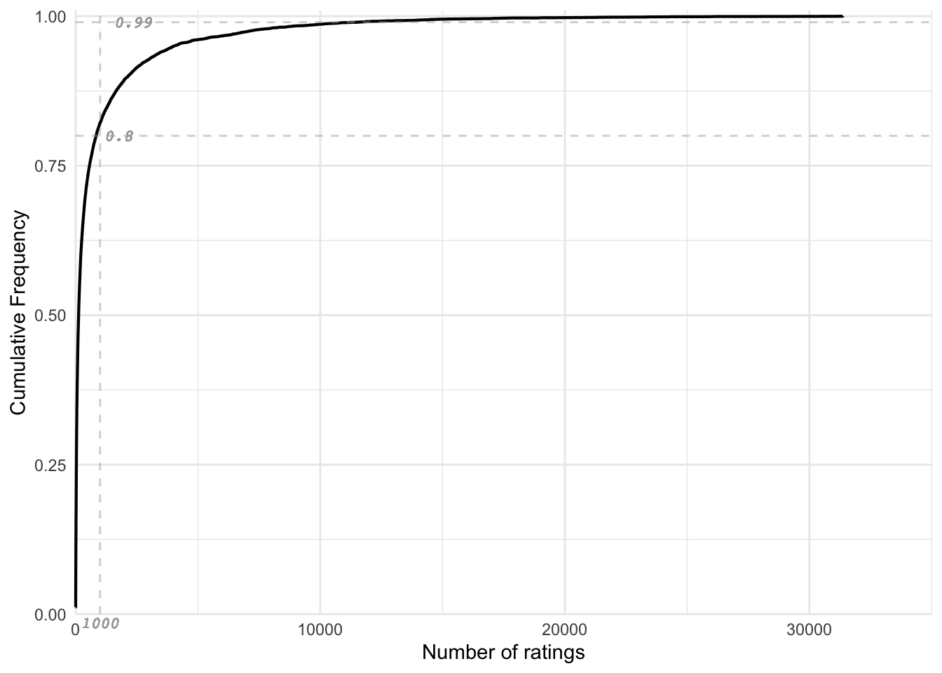
The normalized ECDF is illustrated in Figure 4. Approximately, around 80% of movies have less than 1000 ratings and around 20% movies have more than 1000 ratings; Moreover, 1% of movies have more than 10000 ratings.
Users
We then proceed with users feature. The user details are given by the userId column. We shall check the number of unique users in the dataset.
length(unique(mlens$userId))
## [1] 69878
There are 69878 different users in the mlens dataset. Similar to movie ratings discussed earlier, the number of ratings per user is a large long-tailed distribution and we can use normalized ECDF to accommodate all the data in the plot.
# Density plot of distribution of ratings grouped by userId
mlens %>%
  group_by(userId) %>%
  summarize(num_rating=n()) %>%
  arrange(num_rating) %>%
  ggplot(aes(num_rating)) +
  geom_density() +
  ylab("Density") +
  theme(plot.title = element_text(hjust = 0.5,face="italic"),
        axis.title.x = element_blank(),
        axis.text.x = element_blank(),
        axis.ticks.x = element_blank())
Looking at Figure 5, the distribution appears to be a right skewed distribution, with a few users who have rated a large number of movies and the majority of users have rated few movies.
# Normalized ecdf of the number of ratings per user
mlens %>%
  group_by(userId) %>%
  summarise(num_rating = n()) %>%
  ggplot(aes(x = num_rating)) +
  stat_ecdf(geom = "step",
            size = 0.75,
            pad = FALSE) +
  theme_minimal() +
  coord_cartesian(clip = "off") +
  geom_vline(xintercept = 270, colour = "darkgrey",alpha=0.5,linetype="dashed") +
  geom_text(aes(270, 0, label=270,vjust=1.5),
            size=3,color="darkgrey",family="Courier", fontface="italic") +
  geom_hline(yintercept = 0.90, colour = "darkgrey",alpha=0.5,linetype="dashed") +
  geom_text(aes(0, 0.9, label=0.9,hjust=1.5),
            size=3,color="darkgrey",family="Courier", fontface="italic") +
  scale_x_continuous(limits = c(0,7000),
                     expand = c(0, 0),
                     name="Number of ratings") +
  scale_y_continuous(limits = c(0, 1.01),
                     expand = c(0, 0),
                     name = "Cumulative Frequency") +
  theme(plot.title=element_text(hjust = 0.5,face="italic"),
        axis.text.x = element_text(angle=0))
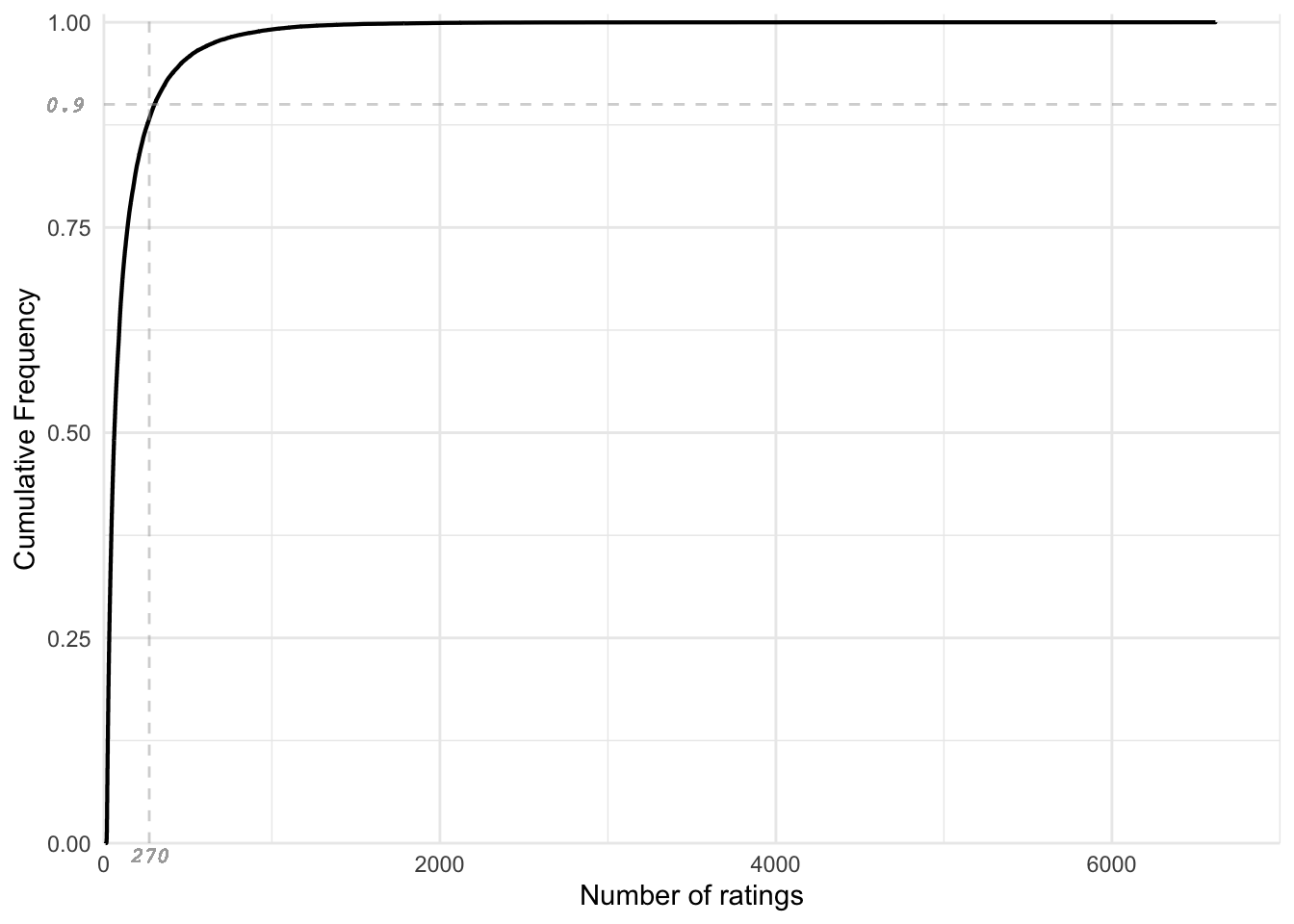
The ECDF plot is illustrated in Figure 6. Approximately 90% of the users have rated less than 300 movies and only a small group of users have ratings exceeding 1000. The ECDF plot illustrates variation in the distribution of data. One of the ways to address such data with high variance in data points is, regularization.
Date
Moving on to the next feature, we explore the effects of date on the ratings, given by the timestamp variable.
# Overview of Year data in mlens
mlens %>%
  mutate(date = date(as_datetime(timestamp, origin="1970-01-01"))) %>%
  mutate(year = year(date)) %>%
  pull(year) %>% unique() %>% sort()
## [1] 1995 1996 1997 1998 1999 2000 2001 2002 2003 2004 2005 2006 2007 2008 2009
The mlens dataset contains ratings from the year 1995 to 2009.
# Average rating by day
mlens %>%
  mutate(Day = day(date(as_datetime(timestamp, origin="1970-01-01")))) %>%
  group_by(Day) %>%
  summarise(avg_rating=mean(rating)) %>%
  ggplot(aes(Day, avg_rating)) +
  geom_point() +
  geom_smooth() +
  xlab("Day of the month") +
  ylab("Average rating") +
  theme(plot.title=element_text(hjust = 0.5,face="italic"))
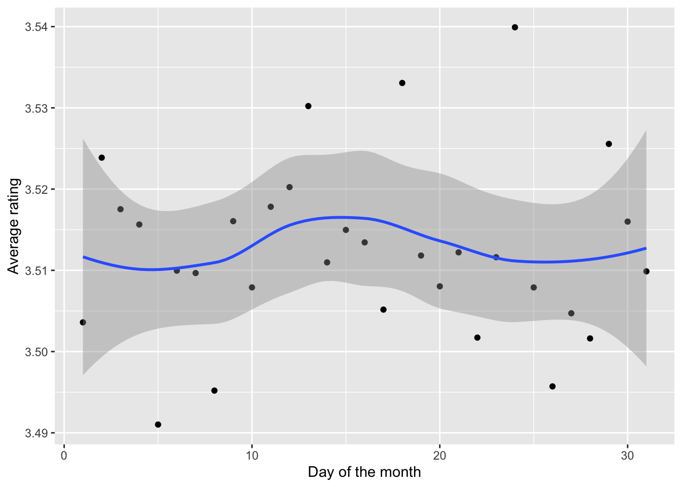
The plot of average rating versus day in Figure 7 accounts for the effect of the day when the rating was given. We see that, there are no extreme variations in the rating due to the day variable. Therefore, we progress to the next variable.
Genres
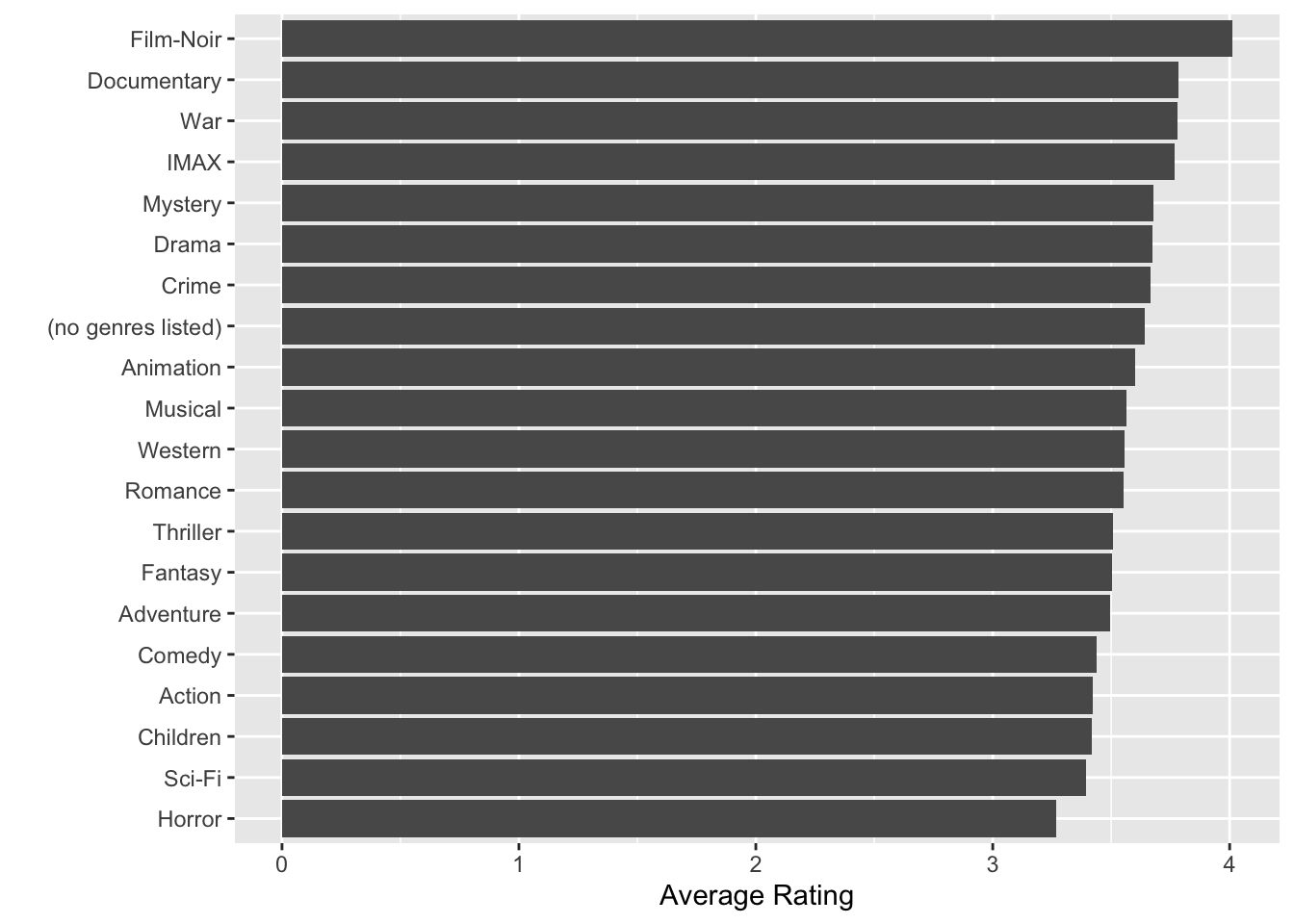
The next variable to analyze is the genres column. The genres column is a column with multiple labels. We have applied one-hot encoding on the genres column to analyze effects of each of the individual genres. We begin our analysis on genre by estimating the average rating for each genre.
# Average rating of movies of each genre
data.frame(avg_rating =
             sapply(names(dplyr::select(encoded_mlens,-all_of(names(mlens)))),
                    function(i){
                    mean(encoded_mlens$rating[as.logical(encoded_mlens[[i]])])})) %>%
  mutate(genre = rownames(.)) %>%
  ggplot(aes(reorder(genre,avg_rating),avg_rating)) +
  geom_bar(stat="identity") +
  coord_flip() +
  xlab("") +
  ylab("Average Rating") +
  theme(plot.title=element_text(hjust = 0.5,face="italic"))
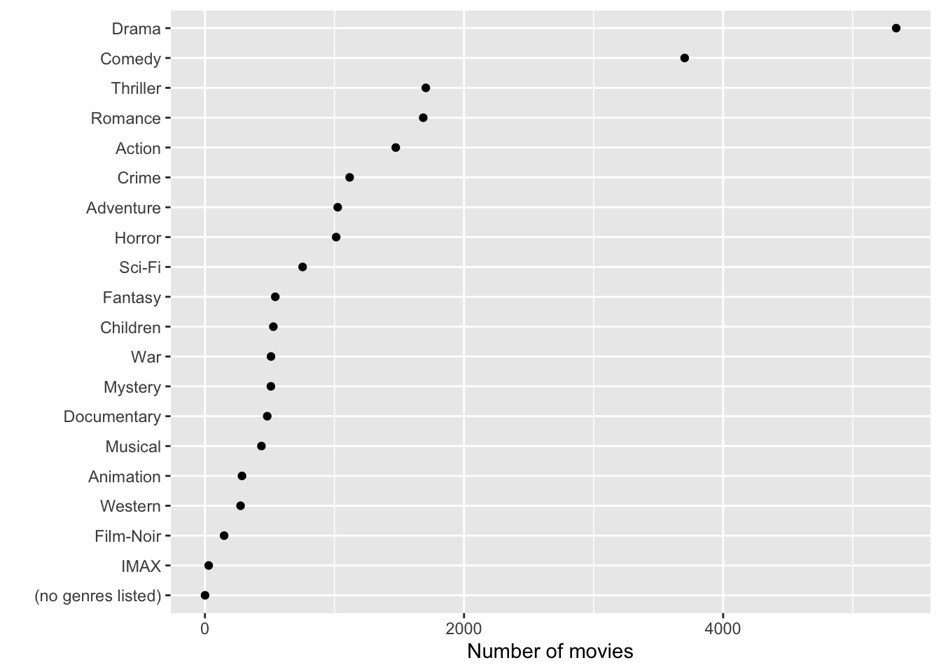
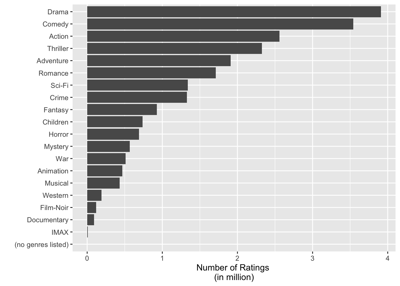
We will now inspect the number of ratings for each genre and the number of movies in each genre.
# Number of movies of each genre
data.frame(num_movies = encoded_mlens %>%
             dplyr::select(-all_of(vars),"movieId") %>%
             distinct() %>%
             colSums()) %>%
  mutate(genre = rownames(.)) %>%
  filter(genre!="movieId") %>%
  ggplot(aes(reorder(genre,num_movies),num_movies)) +
  geom_point() +
  coord_flip() +
  xlab("") +
  ylab("Number of movies") +
  theme(plot.title=element_text(hjust = 0.5,face="italic"))
# Number of ratings of each genre
data.frame(num_ratings = encoded_mlens %>%
                         dplyr::select(-all_of(vars)) %>%
                         colSums()) %>%
  mutate(genre = rownames(.)) %>%
  ggplot(aes(reorder(genre,num_ratings),num_ratings/1000000)) +
  geom_bar(stat="identity") +
  coord_flip() +
  xlab("") +
  ylab("Number of Ratings \n(in million)") +
  theme(plot.title=element_text(hjust = 0.5,face="italic"))
Additionally, genre is not entered for 1 movie among 10677 movies. We need to handle this data; to fix the data or to eliminate it.
Release Year of the Movie
With regards to the mlens dataset, we have release year within the movie title column that can be extracted and analyzed for patterns. We will extract this detail and analyze how movie rating is related to the release year.
# Release Year Patterns
mlens %>%
  mutate(ReleaseYear  = as.numeric(sub("\\).*", "",
                                       sub(".*\\(", "", str_sub(title,-6,-1))))) %>%
  group_by(ReleaseYear) %>%
  summarise(avg_rating=mean(rating)) %>%
  ggplot(aes(ReleaseYear, avg_rating)) +
  geom_point() +
  geom_smooth() +
  xlab("Release Year of movies") +
  ylab("Average rating") +
  theme(plot.title=element_text(hjust = 0.5,face="italic"))
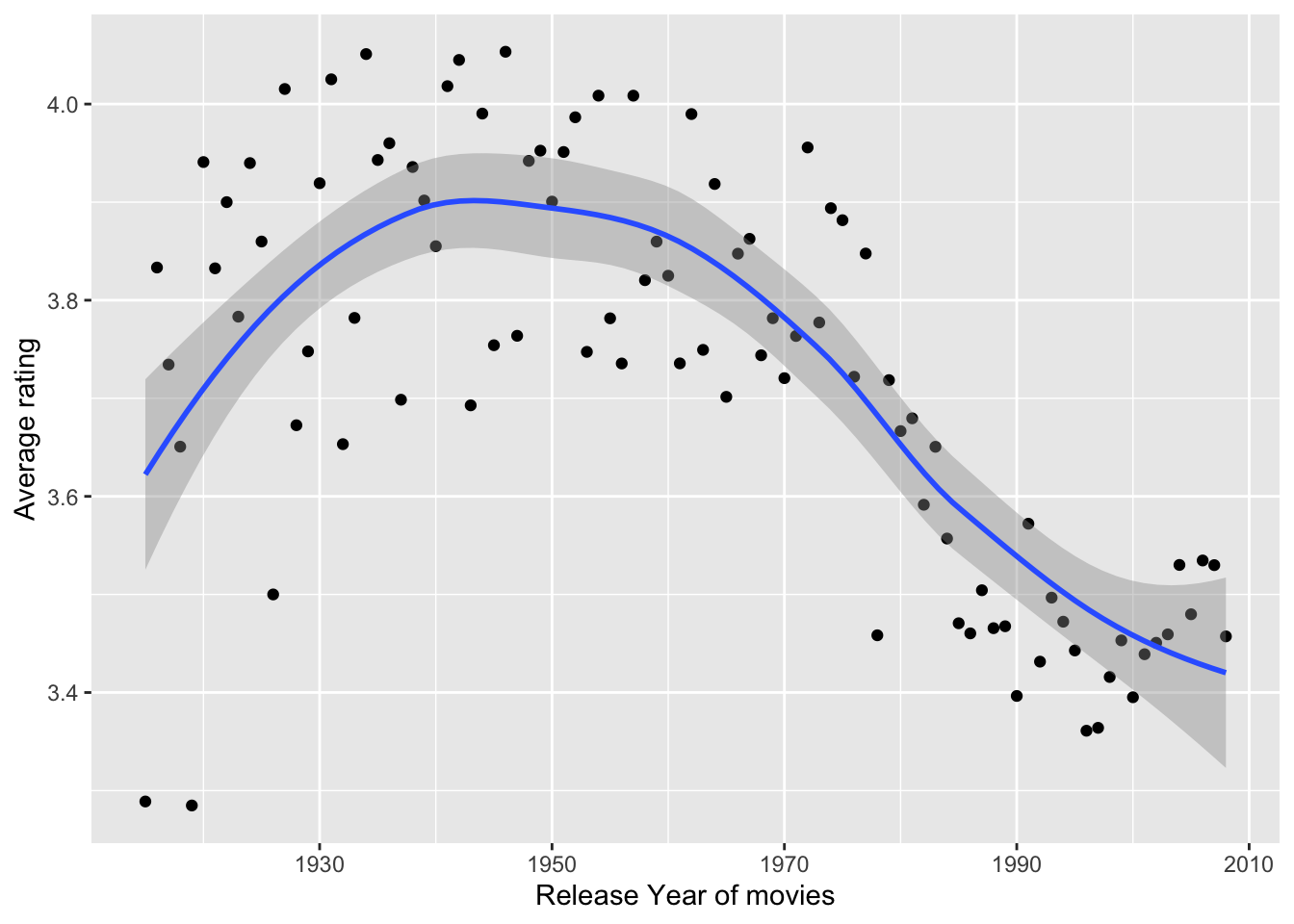
To capture the variance in the data, we could consider the release year in our linear model to account for the effects of the movie release year.
Data Preparation
This is quite an important step before feeding the data to our machine learning algorithm. This step is essential and involves various data preprocessing tasks. As explored in the previous section, we do not have any missing values to handle in mlens dataset. However, there is a data point with “no genres listed” in genre column. A movie will have a genre associated with it and this entry is assumed to be unintentional. Hence, we need to fix this or remove it. We will be removing the following entry to avoid instability in modeling.
##   userId movieId rating  timestamp                title             genres
## 1   7701    8606    5.0 1190806786 Pull My Daisy (1958) (no genres listed)
## 2  10680    8606    4.5 1171170472 Pull My Daisy (1958) (no genres listed)
## 3  29097    8606    2.0 1089648625 Pull My Daisy (1958) (no genres listed)
## 4  46142    8606    3.5 1226518191 Pull My Daisy (1958) (no genres listed)
## 5  57696    8606    4.5 1230588636 Pull My Daisy (1958) (no genres listed)
## 6  64411    8606    3.5 1096732843 Pull My Daisy (1958) (no genres listed)
## 7  67385    8606    2.5 1188277325 Pull My Daisy (1958) (no genres listed)
We then create a 90/10 train-test split of the mlens dataset for our model evaluation purposes. The model is created and trained in the train set and tested in the test set. This is called the prototyping phase that revolves around model selection, which requires measuring the RMSE of plausible candidate models. When we are satisfied with the selected model type and hyperparameters, the last step of the prototyping phase is to train a new model on the entire mlens set using the best hyperparameters found. The model is then validated on data we had put aside, the validation set. This gives us an estimate of the generalization error.i.e how well our model generalizes to new data.
##########################################################
# Create train set, test set
##########################################################
## Create train and test sets for cross validation
# Create train set and test set
set.seed(1, sample.kind="Rounding")
test_index <- createDataPartition(y = mlens$rating, times = 1 ,p=0.1, list = FALSE)
train_set <- mlens[-test_index,]
temp <- mlens[test_index,]

# Make sure userId and movieId in validation set are also in mlens set
test_set <- temp %>%
  semi_join(train_set, by = "movieId") %>%
  semi_join(train_set, by = "userId")

# Add rows removed from validation set back into mlens set
removed <- anti_join(temp, test_set)
train_set <- rbind(train_set, removed)

rm(test_index, temp, removed)
Furthermore, we will encode the train and test set similar to mlens dataset and extract day of the month as well as the release year of the movie from the dataset. The below code implements the necessary data manipulation tasks.
# Extracting Day from timestamp column and Release year of the movie from title column : train_set
train_set <- train_set %>%
  mutate(Day = day(as_datetime(train_set[["timestamp"]]))) %>%
  mutate(ReleaseYear  = as.numeric(sub("\\).*", "", sub(".*\\(", "", str_sub(title,-6,-1)))))

# Extracting Day from timestamp column and Release year of the movie from title column : test_set
test_set <- test_set %>%
  mutate(Day = day(as_datetime(test_set[["timestamp"]]))) %>%
  mutate(ReleaseYear  = as.numeric(sub("\\).*", "", sub(".*\\(", "", str_sub(title,-6,-1)))))

# One-hot encoding on the genres column
train_set <- one_hot_encoding(train_set,"genres","|")
test_set <- one_hot_encoding(test_set,"genres","|")
Model Selection
This is a crucial step of shortlisting promising models where we train different viable models of different categories depending on our data. In this case, we will consider linear model, linear model with regularization and matrix factorization. We will measure and compare the performance of each of these models and analyze the errors.
Linear Model
We are now ready to train a machine learning model on our data. Our first model, is a linear regression model. We begin with a simple prediction of rating movies with an average rating, as described in this formula:
\[Y_{u,i} = \mu + \varepsilon_{u,i}\]where $Y_{u,i}$ is the predicted rating, $\mu$ is the mean of observed ratings and $\varepsilon_{u,i}$ is the error distribution. As per our prior analysis of the variable movieId, we noted that, the variability in the rating can be explained by the movieId. In other words, some movies are more popular than others and hence the rating varies. This is called as movie effect or movie bias. This can be expressed by the formula:
\[Y_{u,i} = \mu + b_i +\varepsilon_{u,i}\]where $Y_{u,i}$ is the predicted rating, $\mu$ is the mean of observed ratings, $b_i$ is the movie bias and $\varepsilon_{u,i}$ is the error distribution. We can estimate the movie bias as the difference between observed rating $y_i$ and the estimated mean $\hat \mu$ as described below:
\[\hat{b}_i = \frac{1}{N}{\sum_{i=1}^{N}{({y_i} - \hat\mu)}}\]where $N$ is the number of ratings per movie, $y_i$ is the actual rating and $\hat\mu$ is the estimated mean of ratings. Similar to the movie effects, different users have different rating patterns. For instance, some users rate all movies with approximately 4 or 5 rating; some users rate all movies with a poor rating. This is termed as the user effect or user bias. This can be described by the formula:
\[Y_{u,i} = \mu + b_i + b_u +\varepsilon_{u,i}\]where $Y_{u,i}$ is the predicted rating, $\mu$ is the mean of observed ratings, $b_i$ is the movie bias, $b_u$ is the user bias and $\varepsilon_{u,i}$ is the error distribution. Just like the movie bias, we can estimate user bias as follows:
\[\hat{b}_u = \frac{1}{N}{\sum_{i=1}^{N}{({y_i} - \hat\mu - \hat{b}_i)}}\]where $N$ is the number of ratings per user, $y_i$ is the actual rating and $\hat\mu$ is the estimated mean of ratings, $\hat b_i$ is the estimated item bias. We then proceed to add day effects to further improve the model. The equation for our model can be described by:
\[Y_{u,i} = \mu + b_i + b_u + b_t +\varepsilon_{u,i}\]where $Y_{u,i}$ is the predicted rating, $\mu$ is the mean of observed ratings, $b_i$ is the movie bias, $b_u$ is the user bias, $b_t$ is the day bias and $\varepsilon_{u,i}$ is the error distribution. We can estimate the day bias as follows:
\[\hat{b}_t = \frac{1}{N}{\sum_{i=1}^{N}{({y_i}-\hat\mu-\hat{b}_i-\hat{b}_u)}}\]where $N$ is the total number of observations for each day, $y_i$ is the actual rating and $\hat\mu$ is the estimated mean of ratings, $\hat b_i$ is the estimated item bias, $\hat b_u$ is the estimated user bias. As per our data exploration, we could use the bias due to release year of the movie. Our model can now be described by:
\[Y_{u,i} = \mu + b_i + b_u + b_t + b_y + \varepsilon_{u,i}\]where $Y_{u,i}$ is the predicted rating, $\mu$ is the mean of observed ratings, $b_i$ is the movie bias, $b_u$ is the user bias, $b_t$ is the day effects, $b_y$ is the bias due to the movie release year and $\varepsilon_{u,i}$ is the error distribution. We can estimate the release year bias as follows:
\[\hat{b}_y = \frac{1}{N}{\sum_{i=1}^{N}{({y_i}-\hat\mu-\hat{b}_i-\hat{b}_u- \hat{b}_t)}}\]where $N$ is the total number of movies released in the year $i$, $y_i$ is the actual rating and $\hat\mu$ is the estimated mean of ratings, $\hat b_i$ is the estimated item bias, $\hat b_u$ is the estimated user bias and $\hat b_t$ is the estimated day bias. To further enhance our model, we will add the genre effect. As per our analysis on genres, we see that some genres tend to have higher rating than the others. We need to estimate the coefficient of each genre. We perform a one-hot encoding on our genres variable. This will result in separate genre variables owing to every individual genre in the mlens dataset.
\[Y_{u,i} = \mu + b_i + b_u + b_t + b_y + g_{u,i} + \varepsilon_{u,i}\]where $Y_{u,i}$ is the predicted rating, $\mu$ is the mean of observed ratings, $b_i$ is the movie bias, $b_u$ is the user bias, $b_t$ is the day effects, $g_{u,i}$ is total genre bias of $k$ genres for a movie $i$, $b_y$ is the bias due to the movie release year and $\varepsilon_{u,i}$ is the error distribution. We can rewrite this $g_{u,i}$ as,
\[g_{u,i} = \sum_{k=1}^{K} x_{u,i}^{k} \beta_k = \alpha + \beta_1x_{u,i}^1 + \beta_2 x_{u,i}^2 + ... +\beta_K x_{u,i}^K\]with $x^k_{u,i} = 1$ if $g_{u,i}$ is of genre $k$, $\beta_k$ are the co-efficients we have to estimate to predict $g_{u,i}$. We estimate the $\beta_k$ by the formula:
\[g_{u,i} = \sum_{k=1}^{K} x_{u,i}^{k}{\beta_k} = ({y_i} - \hat\mu - \hat{b}_i - \hat{b}_u - \hat{b}_t - \hat{b}_y)\]where $\beta_k$ is beta for genre $k$ and $N$ is the number of ratings with $g_{u,i}$ for each of the genre $k$, $\hat b_t$ is the estimated day bias, $\hat b_i$ is the estimated item bias and $\hat b_u$ is the estimated user bias, $\hat b_t$ is the estimated day bias, $\hat b_y$ is the estimated bias due to the release year of the movie. We can estimate coefficients $\beta$ by a simple transformation of the matrix of train set using the concept of Moore-Penrose pseudoinverse.
\[\overrightarrow\beta = (X^T X)^{-1} X^T y\]where $X$ is the matrix of encoded genre columns $y$ is the total genre bias($g_{u,i}$). Basically, we take the transpose of the matrix and multiply by itself. This will yield a square matrix and we take the inverse of this matrix and multiply that by the transpose again. Finally, we estimate coefficients by multiplying this with the dependent variable, in this case, the genre bias $g_{u,i}$.
We have now added item bias, user bias, day bias, release year bias and genre bias as per our exploratory data analysis. Although we are trying to maximize the performance of our model here by minimizing our loss function, there is a tendency of overfitting as we include more and more features. This happens because, we could have unknowingly extracted some noise from the data, even if the noise does not represent the model structure. This is the basis for our next section: Linear Model with Regularization.
Linear Model with Regularization
The motivation behind regularization is simple. The linear model tends to overfit the data when dealing with a very large number of features. This can be avoided by adding a penalty parameter, for constraining the size of the coefficients, such that, the only way the coefficients can increase is if there is a comparable decrease in the model’s loss function.
There are three common penalty parameters: Ridge, Lasso and Elastic Net. The difference between the three is the penalty term that is added to the loss function. The penalty term in case of Lasso regression is referred to as “L1-norm”, and in case of ridge regression it is called “L2-norm”. With regards to regularization of movie effects, ridge regression adds a penalty of $\lambda\sum_i{b_i^2}$ to our previous sum of squared errors (SSE) with movie effects, lasso regression adds a penalty of $\lambda\sum_i{|b_i|}$ to SSE, and elastic net penalizes regression model with both the L1-norm and L2-norm. We will perform ridge regression on our data.
Now, the loss function can be described by the formula:
\[SSE = \sum_{u,i}{(y_i -\hat y_i)^2} + \lambda\sum_i{\hat b_i^2}\]where $\lambda$ is the penalty, $y_i$ is the actual rating, $\hat y_i$ is the estimated rating and $\hat b_i$ is the estimated item bias for $i$ items. In the case of mlens dataset, there are 2 features that need regularization: movieId and userId. The loss function(SSE) with penalty term can be described as follows:
\[\sum_{u,i}{(y_i - \hat\mu - \hat b_i -\hat b_u )^2} + \lambda \left( \sum_i{\hat b_i^2} + \sum_u{\hat b_u^2}\right)\]where $\lambda$ is the penalty, $y_i$ is the actual rating, $\hat y_i$ is the estimated rating , $\hat b_i$ is the estimated item bias for $i$ items and $\hat b_u$ is the estimated user bias for $u$ users. This can be further deduced to estimate $\hat b_i$ using calculus, thereby making the equation:
\[\hat b_i(\lambda) = \frac {1} {\lambda + n_i} {\sum_{j=1}^{n_i}{(y_{u,i}-\hat \mu)}}\]where $n_i$ is the number of ratings given for movie i, $\lambda$ is the penalty, $y_{u,i}$ is the actual rating and $\hat \mu$ is the estimated mean of ratings. Once we estimate $\hat b_i$, we can estimate $\hat b_u$ as
\[\hat b_u(\lambda) = \frac {1} {\lambda + n_u} {\sum_{i=1}^{n_u}{(y_{u,i}-\hat \mu - \hat b_i)}}\]where $n_u$ is the number of ratings given by user u, $\lambda$ is the penalty, $y_{u,i}$ is the actual rating and $\hat \mu$ is the estimated mean of ratings and $\hat b_i$ is the movie bias estimated using regularization. Next, we perform hyperparameter tuning on our model using the regularization parameter $\lambda$ for the best possible RMSE.
We can further enhance our model by adding genre bias to the regularized model with optimal $\lambda$. Now, our model can be described by the formula:
\[\sum_{u,i}{(y_i - \hat\mu - \hat b_i -\hat b_u -\hat g_{u,i} - \hat b_y)^2} + \lambda_{opt} \left( \sum_i{\hat b_i^2} + \sum_u{\hat b_u^2}\right)\]where $\hat g_{u,i}$ is the estimated genre bias, $y_{u,i}$ is the actual rating and $\hat \mu$ is the estimated mean of ratings, $\hat b_i$ is the estimated item bias for $i$ items, $\hat b_u$ is the estimated user bias for $u$ users and $\lambda_{opt}$ is the optimal lambda for the lowest RMSE and $\hat b_y$ is the estimated movie release year bias.
Matrix Factorization
Initially, we discussed on the strategies used in recommender systems and noted that collaborative filtering is more accurate than content based filtering. This is because this technique analyzes user preferences and uses these for providing personalized recommendations to other similar users. Matrix factorization achieves collaborative filtering by approximating an incomplete rating matrix using the product of two matrices in a joint latent factor space of dimensionality $f$.
Before we can get into further details of matrix factorization we will describe some key elements of this technique: The rating matrix, latent factors and the latent vectors.
A rating matrix is a matrix of u(users) by i(items) of explicit user ratings over items. This is generally sparse because, not all users could have watched all movies. An entry (i,j) in this sparse matrix corresponds to the rating, given by user $u$, of an item $i$. The latent vector of factors are inferred features from movie rating patterns of users, and are estimated by minimizing the loss function. Examples for latent factors in the context of movies, can be genre, depth of a character, amount of action, age group of the target audience or can even be completely uninterpretable. These inferred features are often called latent vectors and the k attributes are often called the latent factors.
Suppose each movie $i$ is associated with a vector $q_i$ and user $u$ is associated with a vector $p_u$. Then the rating matrix can be determined by the dot product of $q_i^T$ and $p_u$. For a given item i, the elements of $q_i$ measure the extent to which the item possesses those factors, positive or negative. For a given user u, the elements of $p_u$ measure the extent of interest the user has in items that are high on the corresponding factors, positive or negative.
Therefore, the matrix factorization model can be described by the formula:
\[\hat r_{u,i} = \sum_ {f = 0}^{k\space factors} {p_u q_i^T }\]where $p_u$ is the item’s latent vectors with dimensions $u$ x $k$ , $q_i$ is the user’s latent vectors with dimensions $i$ x $k$, and $\hat r_{u,i}$ gives the user’s overall interest in the item’s characteristics.
Furthermore, the expressive power of the model can be tuned by modifying the number of latent factors.
We can implement the matrix factorization algorithm using alternating least squares(ALS) or stochastic gradient descent(SGD). In the case of mlens dataset, a suitable approach is the SGD compared to the ALS approach because of two reasons. The rating matrix in case of mlens is based on explicit feedback, meaning, the rating is based on the rating of a user on an item.
SGD is rather slow or ineffective and ALS is the preferred approach in case of implicit feedback datasets, where the user preferences are modeled based on search history, purchase history, browsing activity, and therefore the rating matrix cannot be considered sparse.
Model Evaluation
This section presents the code and results of the models discussed in the previous section. We will measure MAE and RMSE for each of the models discussed above. But, we will consider only the root-mean-square error (RMSE) for model selection.
Linear Model
Initial Prediction
We start building our recommender system by predicting the same rating for all movies irrespective of the user. The initial prediction is given by the average of ratings $\mu$:
\[Y_{u,i} = \mu + \varepsilon_{u,i}\]where $Y_{u,i}$ is the predicted rating, $\mu$ is the mean of observed ratings and $\varepsilon_{u,i}$ is the error distribution.
# Average rating as the predicted rating
mu <- mean(train_set$rating)
# Predictions with test set for the first model
naive_rmse <- RMSE(test_set$rating, mu)
naive_mae <- MAE(test_set$rating, mu)
## method	          RMSE         MAE
## Average rating	  1.059683     0.8549174
We can improve this model by adding movie effects as per our previous discussion.
Include Movie effects
Next, we include movie effects to our model. The user ratings can now be described by,
\[Y_{u,i} = \mu + b_i +\varepsilon_{u,i}\]where $Y_{u,i}$ is the predicted rating, $\mu$ is the mean of observed ratings, $b_i$ is the movie bias and $\varepsilon_{u,i}$ is the error distribution.
# Estimation of Movie bias
movie_avgs <- train_set %>%
  group_by(movieId) %>%
  summarize(b_i = mean(rating - mu))
# Predictions on test set with estimated movie bias
preds_movie <- mu + test_set %>%
  left_join(movie_avgs, by='movieId') %>%
  pull(b_i)
# Calculating RMSE for the model with Movie effects
rmse_movie <- RMSE(test_set$rating,preds_movie)
# Calculating MAE for the model with Movie effects
mae_movie <- MAE(test_set$rating,preds_movie)
## method                  RMSE         MAE
## Average rating       1.059683      0.8549174
## Movie Effects        0.9430407     0.7375076
We note that, the RMSE and MAE improved by adding movie effects.
Include User effects
Then, we include user effects to the model. The user ratings can now be given by,
\[Y_{u,i} = \mu + b_i + b_u +\varepsilon_{u,i}\]where $Y_{u,i}$ is the predicted rating, $\mu$ is the mean of observed ratings, $b_i$ is the movie bias, $b_u$ is the user bias and $\varepsilon_{u,i}$ is the error distribution.
# Estimation of User bias
user_avgs <- train_set %>%
  left_join(movie_avgs, by='movieId') %>%
  group_by(userId) %>%
  summarize(b_u = mean(rating - mu - b_i))
# Predictions on test set with estimated movie and user bias
preds_movie_user <- test_set %>%
  left_join(movie_avgs, by='movieId') %>%
  left_join(user_avgs, by='userId') %>%
  mutate(pred = mu + b_i + b_u) %>%
  pull(pred)
# Calculating rmse and mae for the model with Movie and User effects
rmse_movie_user <- RMSE(test_set$rating,preds_movie_user)
mae_movie_user <- MAE(test_set$rating,preds_movie_user)
## method                 RMSE          MAE
## Average rating         1.059683      0.8549174
## Movie Effects          0.9430407     0.7375076
## Movie + User Effects   0.8646879     0.6686567
We observe further reduction in our loss function. Therefore, we continue with our model, including the movie and the user effects.
Include Day effects
As per our previous analysis, we include day effects to the model. The user ratings can now be described by the following equation:
\[Y_{u,i} = \mu + b_i + b_u + b_t + \varepsilon_{u,i}\]where $Y_{u,i}$ is the predicted rating, $\mu$ is the mean of observed ratings, $b_i$ is the movie bias,$b_u$ is the user bias, $b_t$ is the day bias and $\varepsilon_{u,i}$ is the error distribution. This code extends the linear modeling from earlier to include the day effects in the model.
# Estimation of day effects
day_avgs <- train_set %>%
  left_join(movie_avgs, by='movieId') %>%
  left_join(user_avgs, by='userId') %>%
  group_by(Day) %>%
  summarize(b_t = mean(rating - mu - b_i - b_u))
# Smoothing the values of b_t
f_smooth <- loess(b_t ~ Day,data = day_avgs,family="gaussian",span=1)
# Predictions on test set with estimated movie, user and day bias
preds_movie_user_day <- test_set %>%
  left_join(movie_avgs, by='movieId') %>%
  left_join(user_avgs, by='userId') %>%
  mutate(pred = mu + b_i + b_u  + f_smooth$fitted[Day]) %>%
  pull(pred)
# Calculating rmse and mae for the model with Movie, User and Day effects
rmse_movie_user_day <- RMSE(test_set$rating,preds_movie_user_day)
mae_movie_user_day <- MAE(test_set$rating,preds_movie_user_day)
## method                        RMSE          MAE
## Average rating                1.059683      0.8549174
## Movie Effects                 0.9430407     0.7375076
## Movie + User Effects          0.8646879     0.6686567
## Movie + User + Day Effects	 0.8646880     0.6686560
We see no improvement in RMSE after adding the day effects. Hence, we continue modeling for genre effects in our linear model along with movie effects and user effects only.
Include Release Year effects
We continue our model, to evaluate the effects due to the release year of the movie. Now the model can be described by:
\[Y_{u,i} = \mu + b_i + b_u + b_y + \varepsilon_{u,i}\]where $Y_{u,i}$ is the predicted rating, $\mu$ is the mean of observed ratings, $b_i$ is the movie bias, $b_u$ is the user bias, $b_y$ is the bias due to the movie release year and $\varepsilon_{u,i}$ is the error distribution. This code takes the same approach as before, but adds the movie release year effects to the model.
# Estimation of release year effects
relyear_avgs <- train_set %>%
  left_join(movie_avgs, by='movieId') %>%
  left_join(user_avgs, by='userId') %>%
  group_by(ReleaseYear) %>%
  summarize(b_ry = mean(rating - mu - b_i - b_u))
# Predictions on test set with estimated movie, user, day and release year bias
preds_movie_user_relyear <- test_set %>%
  left_join(movie_avgs, by='movieId') %>%
  left_join(user_avgs, by='userId') %>%
  left_join(relyear_avgs, by='ReleaseYear') %>%
  mutate(pred = mu + b_i + b_u + b_ry) %>%
  pull(pred)
# Calculating rmse and mae for the model with Movie, User and Day effects
rmse_movie_user_relyear <- RMSE(test_set$rating,preds_movie_user_relyear)
mae_movie_user_relyear <- MAE(test_set$rating,preds_movie_user_relyear)
## method                                RMSE          MAE
## Average rating                        1.059683      0.8549174
## Movie Effects                         0.9430407     0.7375076
## Movie + User Effects                  0.8646879     0.6686567
## Movie + User + Day Effects            0.8646880     0.6686560
## Movie + User + Release Year Effects	 0.8643204     0.6680288
Include Genre effects
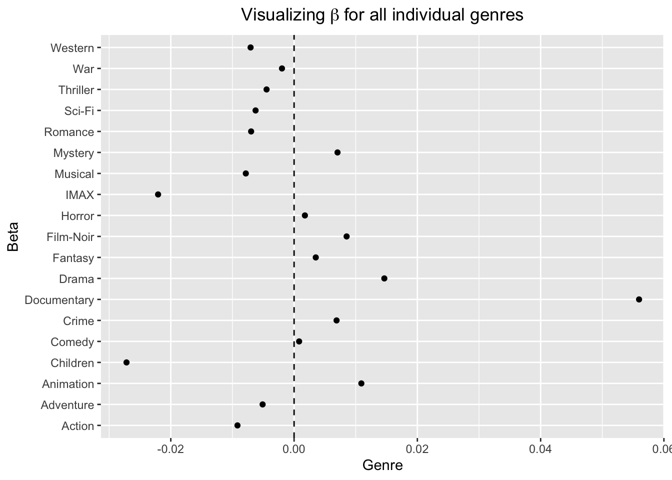
We then proceed to include the genre effects. The equation for our model can be described by:
\[Y_{u,i} = \mu + b_i + b_u + b_y + g_{u,i} + \varepsilon_{u,i}\]where $Y_{u,i}$ is the predicted rating, $\mu$ is the mean of observed ratings, $b_i$ is the movie bias, $b_u$ is the user bias, $g_{u,i}$ is total genre bias of $k$ genres for a movie $i$, $b_y$ is the bias due to the movie release year and $\varepsilon_{u,i}$ is the error distribution. As discussed in the previous section, we have used one-hot encoding on the multilabel genres column and we will estimate the coefficients $\beta$ for all the individual genres using the concept of Moore-Penrose pseudouniverse to estimate the genre bias. We use the MASS package that provides a calculation of the Moore–Penrose inverse through the ginv function. This function calculates pseudoinverse using the singular value decomposition provided by the svd function in the base R package.
# Installing required package for ginv()
if(!require(MASS)) install.packages("MASS", repos = "http://cran.us.r-project.org")
# Note that MASS library has a select function; Use dplyr::select for using select function from dplyr
library(MASS)

# Estimating bias due to genre and genre columns
genre_df <-
  train_set %>%
  left_join(movie_avgs, by='movieId') %>%
  left_join(user_avgs, by='userId') %>%
  left_join(relyear_avgs, by='ReleaseYear') %>%
  mutate(g_ui = rating - mu - b_i - b_u - b_ry) %>%
  dplyr::select(-all_of(vars),-any_of(c("b_i","b_u","b_ry","Day","ReleaseYear")),"g_ui")
# Converting training data to matrix form
x <- as.matrix(genre_df[,-c("g_ui")])
y <- as.matrix(genre_df[,c("g_ui")])
# Estimating co-efficient of individual genres using Moore-Penrose pseudoinverse
beta_df <- data.frame(
  beta =  ginv(x) %*% y,
  genre = names(genre_df[,-c("g_ui")]))
# Estimating predictions for genre effects
g_ui_hat <- rowSums(sapply(beta_df$genre,
                           function(i){
                             as.numeric(beta_df[,1][beta_df$genre==i]) * test_set[[i]]
                           }))
# Plotting coefficients for all genres
  beta_df %>%
  setnames(c("beta","genre")) %>%
  ggplot(aes(beta,genre)) +
  geom_point() +
  geom_vline(xintercept=0, linetype=2) +
  xlab("Genre") +
  ylab("Beta") +
  ggtitle(expression("Visualizing" ~ beta ~ "for all individual genres")) +
  theme(plot.title=element_text(hjust = 0.5,face="italic"))
# Estimating rating predictions
preds_movie_user_day_genre <- test_set %>%
  left_join(movie_avgs, by='movieId') %>%
  left_join(user_avgs, by='userId') %>%
  left_join(relyear_avgs, by='ReleaseYear') %>%
  cbind(g_ui_hat) %>%
  mutate(pred = mu + b_i + b_u + g_ui_hat + b_ry ) %>%
  pull(pred)
# Calculating rmse and mae for the model with Movie, User and genre effects
rmse_genre <- RMSE(test_set$rating,preds_movie_user_day_genre)
mae_genre <- MAE(test_set$rating,preds_movie_user_day_genre)
We see that, the addition of genre effects has further improved the RMSE. In the preceding code chunks, we added features one at a time , measured the RMSE after each addition and cut the ones that did not improve our RMSE. We also note that, the RMSE improved with each of the feature additions except for day of the rating.
## method                                       RMSE          MAE
## Average rating                               1.059683      0.8549174
## Movie Effects                                0.9430407     0.7375076
## Movie + User Effects                         0.8646879     0.6686567
## Movie + User + Day Effects                   0.8646880     0.6686560
## Movie + User + Release Year Effects          0.8643204     0.6680288
## Movie + User + Release Year + Genre Effects	0.8641883     0.6678188
Regularization
Regularization of item and user efffects
We will now compute the regularized estimates of $b_i$ and $b_u$ and predict the rating to minimize the squared errors given by:
\[\sum_{u,i}{(y_i - \hat\mu - \hat b_i -\hat b_u )^2} + \lambda \left( \sum_i{\hat b_i^2} + \sum_u{\hat b_u^2}\right)\]# Optimize lambda by minimizing RMSE
lambdas <- seq(1, 10, 0.25)
mu <- mean(train_set$rating)
rmses <- sapply(lambdas, function(l){
b_i <- train_set %>%
group_by(movieId) %>%
summarize(b_i = sum(rating - mu)/(n()+l))
b_u <- train_set %>%
left_join(b_i, by="movieId") %>%
group_by(userId) %>%
summarize(b_u = sum(rating - mu - b_i)/(n()+l))
preds_reglrzed_movie_user <- test_set %>%
left_join(b_i, by='movieId') %>%
left_join(b_u, by='userId') %>%
mutate(pred = mu + b_i + b_u ) %>%
pull(pred)
return(RMSE(test_set$rating,preds_reglrzed_movie_user))
})
# Visualizing RMSE over a sequence of lambda values
qplot(lambdas, rmses)  +
  theme(plot.title = element_text(hjust = 0.5,face="italic"))
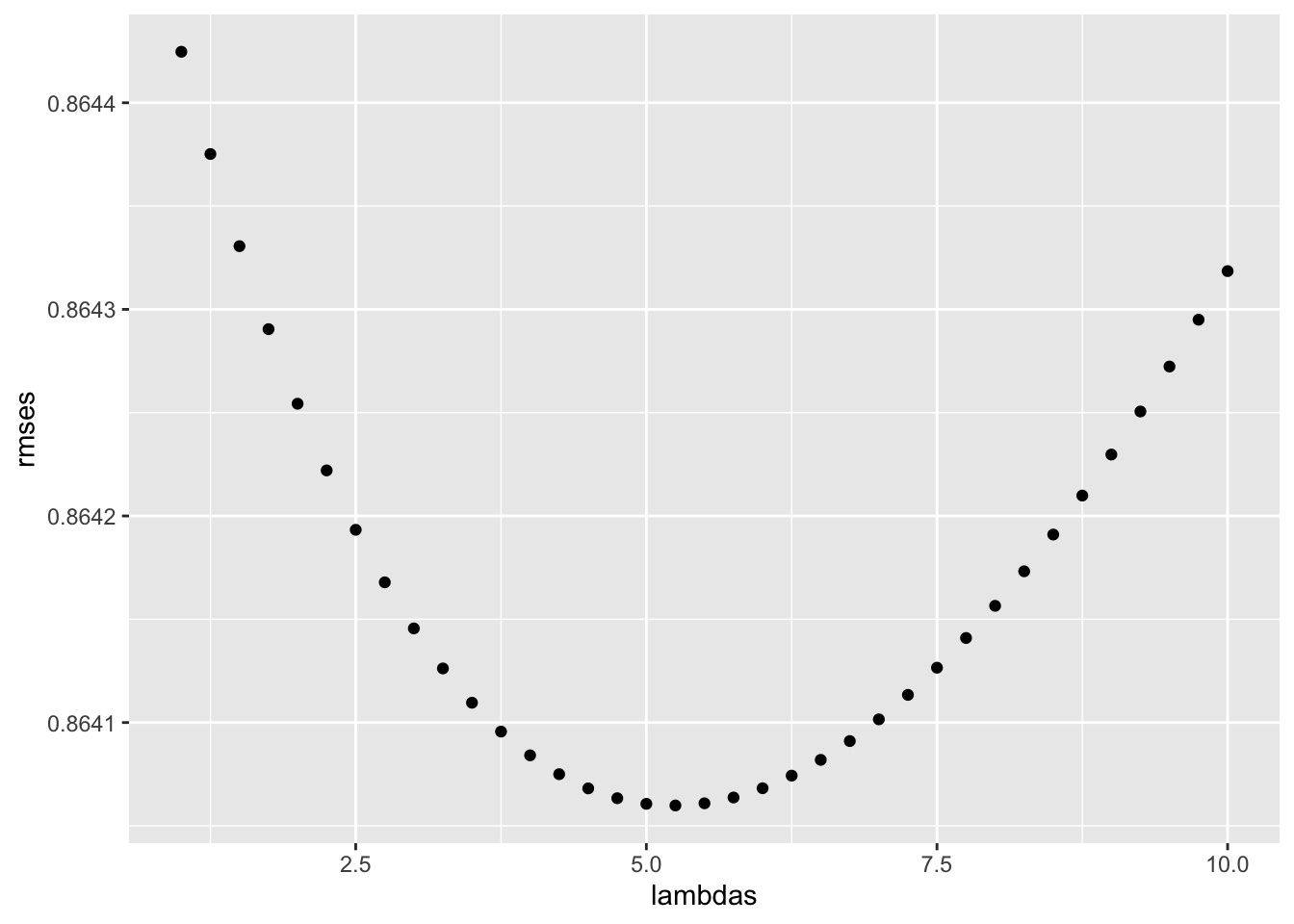
# Optimal lambda for minimizing rmse
lambda <- lambdas[which.min(rmses)]
# Deleting used objects and variables
rm(lambdas,rmses)
### Regularized model with optimal lambda
b_i <- train_set %>%
  group_by(movieId) %>%
  summarize(b_i = sum(rating - mu)/(n()+lambda))
b_u <- train_set %>%
  left_join(b_i, by="movieId") %>%
  group_by(userId) %>%
  summarize(b_u = sum(rating - mu - b_i)/(n()+lambda))
preds_reglrzed_movie_user <- test_set %>%
  left_join(b_i, by='movieId') %>%
  left_join(b_u, by='userId') %>%
  mutate(pred = mu + b_i + b_u) %>%
  pull(pred)
rmse_reglrzed_movie_user <- RMSE(test_set$rating,preds_reglrzed_movie_user)
mae_reglrzed_movie_user <- MAE(test_set$rating,preds_reglrzed_movie_user)
## method                                       RMSE          MAE
## Average rating                               1.059683      0.8549174
## Movie Effects                                0.9430407     0.7375076
## Movie + User Effects                         0.8646879     0.6686567
## Movie + User + Day Effects                   0.8646880     0.6686560
## Movie + User + Release Year Effects          0.8643204     0.6680288
## Movie + User + Release Year + Genre Effects	0.8641883     0.6678188
## Regularized Movie + User                     0.8640599     0.6689203
We see that, our model chose an optimal penalty parameter of 5.25. The results indicate that, the regularization of item and user effects with a penalty parameter of 5.25 yielded improved predicted ratings, resulting in a RMSE of 0.86406 and MAE of 0.66892.
Including genre effects and release year effects to regularized item and user effects
The regularized model outperforms linear model, even without adding any other features. We earlier saw that improvement in RMSE was quite substantial when we added release year and genre effects to our model. To improve the regularized model, we will include the genre effects and release year effects. We do not include day effects, since the RMSE improvement in case of day effects was quite low.
The following code accomplishes the same by implementing model whose squared errors can be described by:
\[\sum_{u,i}{(y_i - \hat\mu - \hat b_i -\hat b_u -\hat g_{u,i} - \hat b_y)^2} + \lambda \left( \sum_i{\hat b_i^2} + \sum_u{\hat b_u^2}\right)\]# Estimating release year bias
b_ry <- train_set %>%
left_join(b_i, by='movieId') %>%
left_join(b_u, by='userId') %>%
group_by(ReleaseYear) %>%
summarize(b_ry = mean(rating - mu - b_i - b_u ))
# Estimating bias due to genre and genre columns
genre_df_reg <-
train_set %>%
left_join(b_i, by='movieId') %>%
left_join(b_u, by='userId') %>%
left_join(b_ry, by='ReleaseYear') %>%
mutate(g_ui = rating - mu - b_i - b_u - b_ry ) %>%
dplyr::select(-all_of(vars),-any_of(c("b_i","b_u","Day","b_ry","ReleaseYear")),"g_ui")
# Converting training data to matrix form
x <- as.matrix(genre_df_reg[,-c("g_ui")])
y <- as.matrix(genre_df_reg[,c("g_ui")])
# Estimating co-efficient of individual genres using Moore-Penrose pseudoinverse
beta_df_reg <- data.frame(
beta = ginv(x) %*% y,
genre = names(genre_df_reg[,-c("g_ui")]))
# Visualizing coefficients of genre with regularized model
beta_df_reg %>%
setnames(c("beta","genre")) %>%
ggplot(aes(beta,genre)) +
geom_point() +
geom_vline(xintercept=0, linetype=2) +
xlab("Genre") +
ylab("Beta") +
ggtitle(expression("Visualizing" ~ beta ~ "for all individual genres")) +
theme(plot.title=element_text(hjust = 0.5,face="italic"))
# Estimating predictions for genre effects
g_ui_hat_reg <- rowSums(sapply(beta_df_reg$genre,
function(i){
as.numeric(beta_df_reg[,1][beta_df_reg$genre==i]) * test_set[[i]]
}))
# Estimating rating predictions
preds_regularized_iu_genre <- test_set %>%
left_join(b_i, by='movieId') %>%
left_join(b_u, by='userId') %>%
left_join(b_ry, by='ReleaseYear') %>%
cbind(g_ui_hat_reg) %>%
mutate(pred = mu + b_i + b_u + b_ry + g_ui_hat_reg) %>%
pull(pred)
# Calculating rmse and mae for the model with Movie, User and genre effects
rmse_genre_reg <- RMSE(test_set$rating,preds_regularized_iu_genre)
mae_genre_reg <- MAE(test_set$rating,preds_regularized_iu_genre)
## method                                                     RMSE          MAE
## Average rating                                             1.059683      0.8549174
## Movie Effects                                              0.9430407     0.7375076
## Movie + User Effects                                       0.8646879     0.6686567
## Movie + User + Day Effects                                 0.8646880     0.6686560
## Movie + User + Release Year Effects                        0.8643204     0.6680288
## Movie + User + Release Year + Genre Effects	              0.8641883     0.6678188
## Regularized Movie + User                                   0.8640599     0.6689203
## Regularized Movie & User + Genre + Release year Effects    0.8636279	    0.6679687
We note that, the RMSE on the regularized model with genre effects and release year effects further reduces to 0.86363 on the test set and the MAE is 0.66797. We observe that, regularization only improves the generalization performance: the performance on the new or unseen data, and does not always guarantee high accuracy. Hence, we turn our focus towards methods that can provide better prediction and are better suited for recommender systems.
Matrix Factorization with stochastic gradient descent
In this section, we implement the matrix factorization technique with stochastic gradient descent using recosystem package. The recosystem package allows for parallel computation and can significantly reduce memory usage. We opted for selection of tuning parameters from a set of candidate values and the following block of code implements matrix factorization.
# Installing recosystem pkg
if(!require(recosystem)) install.packages("recosystem", repos = "http://cran.us.r-project.org")
# Loading recosystem library for recommender object
library(recosystem)
## Collaborative filtering using Matrix Factorization
train_vector <- data_memory(user_index = train_set$userId,
                            item_index = train_set$movieId,
                            rating = train_set$rating,
                            index1=T)
test_vector <- data_memory(user_index = test_set$userId,
                           item_index = test_set$movieId,
                           rating = test_set$rating,
                           index1=T)
# Constructing a Recommender System Object
recommender = recosystem::Reco()
#  Uses cross validation to tune the model parameters
opts <- recommender$tune(train_vector,
                         opts = list(dim = c(10, 20, 30),
                                     lrate = c(0.1, 0.2), # learning rate
                                     costp_l1 = 0,  # L1 regularization cost for user factors
                                     costq_l1 = 0, # L1 regularization cost for item factors
                                     costp_l2 = c(0.01,0.1), # L2 regularization cost for user factors
                                     costq_l2 = c(0.01,0.1), # L2 regularization cost for item factors
                                     nthread = 4,  # number of threads for Parallel computation
                                     niter = 10)) # whether to show detailed information.
# Trains a recommender model with the training data source
recommender$train(train_vector,opts = c(opts$min,
                                        nthread = 4,
                                        niter = 300,
                                        verbose = FALSE))
# Predicts unknown entries in the rating matrix
preds_matrix_fact <- recommender$predict(test_vector, out_memory())
# Estimating rmse and mae for the matrix factorization model
rmse_matrix_fact <- RMSE(test_set$rating, preds_matrix_fact)
mae_matrix_fact <- MAE(test_set$rating, preds_matrix_fact)
## method                                                     RMSE          MAE
## Average rating                                             1.059683      0.8549174
## Movie Effects                                              0.9430407     0.7375076
## Movie + User Effects                                       0.8646879     0.6686567
## Movie + User + Day Effects                                 0.8646880     0.6686560
## Movie + User + Release Year Effects                        0.8643204     0.6680288
## Movie + User + Release Year + Genre Effects	              0.8641883     0.6678188
## Regularized Movie + User                                   0.8640599     0.6689203
## Regularized Movie & User + Genre + Release year Effects    0.8636279	    0.6679687
## Matrix Factorization (recosystem package)                  0.7905278     0.6059103
The results show that the matrix factorization is a powerful approach for implementing recommender systems. The RMSE achieved using this approach corresponds to the lowest RMSE on the test set compared to all other models discussed so far. The RMSE achieved with this approach is 0.79053 and MAE is 0.60591 on the test set.
Final Validation
Once we are confident about our final model, we measure RMSE on the validation set, to estimate the generalization error. This is the last step of prototyping phase where we will train a new model on the entire mlens set using the best hyperparameters found.
In the case of MovieLens 10M set, the finalized model is matrix factorization using recosystem package. This by far, achieves the best RMSE on the test set. Now, we train the complete model with the mlens dataset and estimate the RMSE on validation set.
#######################################################################
# RMSE of finalized model(Matrix Factorization) with the validation set
#######################################################################
# Set random seed
set.seed(1234, sample.kind = "Rounding")
# Convert 'mlens' and 'validation' sets to recosystem input format
mlens_vector <- data_memory(user_index = mlens$userId,
                          item_index = mlens$movieId,
                          rating = mlens$rating,
                          index1=T)
validation_vector <- data_memory(user_index = validation$userId,
                                 item_index = validation$movieId,
                                 rating = validation$rating,
                                 index1=T)
# Create the model object
recommender <- Reco()
# Train the model
recommender$train(mlens_vector,opts = c(opts$min,
                                      nthread = 4,
                                      niter = 300,
                                      verbose = FALSE))
# Estimating predictions using recommender
preds_validation <- recommender$predict(validation_vector, out_memory())
# RMSE for matrix factorization
rmse_validation <- RMSE(validation$rating, preds_validation)
mae_validation <- MAE(validation$rating, preds_validation)

# Tabulating the validation results
rmse_validation_results <- tibble("Final Model" = "Matrix Factorization",
                                  "RMSE on Validation Set" = rmse_validation,
                                  "MAE on Validation Set" = mae_validation)
The matrix factorization achieves similar results on the validation set as well.
## Method (Validation)  RMSE         MAE
## Matrix Factorization	0.7845124    0.6015874
Conclusion
In this project, we examined various strategies to model recommender systems. We discussed linear model, regularization of the relevant features and finally matrix factorization using stochastic gradient descent. The collaborative filtering strategy performs the best among all the models considered, and offers advantages of serendipity to users, and the latent factors are automatically learned without any manual intervention.
Yet, there are quite a few drawbacks of this strategy. One of the typical drawbacks of collaborative filtering system is the cold start problem, that is, dealing with new users and new items with no ratings at all. However, to address this issue, we can develop hybrid models with collaborative filtering for existing users with content based approach on the new users entering the system.
Another disadvantage with collaborative filtering systems is that, it considers only positive user signals based on the options presented. For instance, if a user is presented with option A, B and C and the user selects A, its quite essential to note that the user rejected B and C. Estimating recommendations based only the selection of A, can affect the quality of recommendations made to the user. Therefore, there is immense scope for improvement in the models discussed in this project. However, building a collaborative filtering system for a more advanced recommendation solution requires heavy engineering resources and is not feasible with a commodity computer.
References
(1) F. Maxwell Harper and Joseph A. Konstan. 2015. The MovieLens Datasets: History and Context. ACM Trans. Interact. Intell. Syst. 5, 4, Article 19 (January 2016), 19 pages. DOI:https://doi.org/10.1145/2827872
(2) Rafael A. Irizarry (2020), Introduction to Data Science: Data Analysis and Prediction Algorithms, https://rafalab.github.io/dsbook/
(3) Yixuan Qiu (2020), recosystem: Recommender System Using Parallel Matrix Factorization, https://cran.r-project.org/web/packages/recosystem/vignettes/introduction.html
(4) Y. Koren, R. Bell and C. Volinsky (2009),Matrix Factorization Techniques for Recommender Systems, in Computer, vol. 42, no. 8, pp. 30-37}, Aug 2009. https://doi.org/10.1109/MC.2009.263.
(5) Koren Y., Bell R. (2011),Advances in Collaborative Filtering. In: Ricci F., Rokach L., Shapira B., Kantor P. (eds) Recommender Systems Handbook, Springer, Boston, MA.